Recursive Integration

Question

I'd like to evaluate the following recursive integration using Mathematica

$$ \ M(T) = \int_0^T\int_0^\infty e^{-\delta s}g(x,s)dxds\ +\int_0^T e^{-\delta s}f(s)M(T-s)ds\, $$

where $g(x,s)$ and $f(s)$ are statistical probability density functions. Since it's a recursive function, the initial condition is given by $M(0) = 0$.

For simplicity we can assume $f(s)$ to be an exponential PDF and $g(x,s)$ to be a Farlie–Gumbel–Morgenstern Copula PDF.

I am not interested in the closed form solution of $M(T)$, rather I am interested only in its numerical answer. This is what I've tried so far:

FGMExpExp = Exp[-2 (s + 10 x)] (36. - 18. Exp[s] + Exp[10 x] (-18.  + 19. Exp[s]));
Delta = 0.04; a = 10; b = 1; 
M[0] = 0; (* Initial Condition *)

Mu[T_] := Mu[T] = NIntegrate[Exp[-Delta*s]*x FGMExpExp, {x, 0, 1.05}, {s, 0, T}] + 
    NIntegrate[b Exp[-(Delta + b)*(T - s)] Mu[s], {s,0, T}]   (* Defining the integration *)
Mu[1] (* The quantity we are interested in. Will change T=1 to T=5 later *)

Your help is greatly appreciated.

Answer 1

I am not interested in the closed form solution of M(T) - and that's a great pity, since your equation can be solved exactly by using Laplace transform - for the numbers you have, and in the general case you can go a long way using the same approach.

Analytical solution

Applying Laplace transform to both sides of your equation, $\int_{0}^{\infty}e^{-p T}f(T)dT$, you get

$$\mu(p) = \int_{0}^{\infty}dT\int_{0}^{T}ds\, e^{-\delta s - p t}\tilde{g}(s)+\int_{0}^{\infty}dT\int{0}^{T}ds\, e^{-\delta s - p t}f(s)M(T-s)$$

where $\mu(p)$ is the Laplace transform of $M(T)$, and $\tilde{g}(s) = \int_{0}^{\infty} g(x,s)dx$. Now we can change the order of integrations as

$$\int_{0}^{\infty}dT\int_{0}^{T}ds \rightarrow \int_{0}^{\infty}ds\int_{s}^{\infty}dT$$

assuming, of course, decent behavior of our functions. Your equation then can be rewritten as

$$\mu(p) = \frac{1}{p}\int_{0}^{\infty}ds\, e^{-(p+\delta)s}\tilde{g}(s)+\int_{0}^{\infty}e^{-\delta s}f(s)ds\int_{s}^{\infty}M(T-s)e^{-p T}dT$$

In the last integral, you can shift the integration variable as $T^\prime = T-s $, which will lead for it to $\mu(p)F(p+\delta)$, where F is a Laplace transform for f:

$$F(q) = \int_{0}^{\infty}e^{-q s}f(s)ds$$.

The final form for an equation for $\mu(p)$ is then

$$\mu(p) = \frac{1}{p} G(p+\delta) + \mu(p) F(p+\delta)$$

where $G$ is a Laplace transform of $\tilde{g}$, and I repeat the definition of $F$ for consistency:

$$F(q) = \int_{0}^{\infty}e^{-q s}f(s)ds,\ G(q) = \int_{0}^{\infty}e^{-q s}\tilde{g}(s)ds$$

The solution for this simple algebraic equation is:

$$\mu(p) = \frac{G(p+\delta)}{p(1- F(p+\delta))}$$

This is all there is to it, you just have to invert the Laplace transform.

In practice, if the analytical form of the inverse is hard to get, you can note that here you have a product of 3 functions $1/p$, $G(p+\delta)$, and $1/(1-F(p+\delta))$, for which it is much easier to get the inverses (we actually know them for the first two, only the last one may be a bit problematic). Then, you can use the property of Laplace transform that product in p-space translates into contraction $\int_{0}^{T}dtf(t)g(T-t)$ in T-space. But in your particular example, this is not needed.

Computation and numerics

Clearing some variables:

ClearAll[f,g,a,b,delta,gintx,s,p,mL,fL,mAn,mnum]

We first define your g function as

g[x_, s_] := Exp[-2 (s + 10 x)] (36. - 18. Exp[s] + Exp[10 x] (-18. + 19. Exp[s]))

It turns out to be quite nice:

gintx[s_] = Integrate[g[x, s], {x, 0, Infinity}]

(* 1. E^-s *)

where gintx is what I denoted as $\tilde{g}$ before. Now, its Laplace transform is trivial:

gl[p_]=LaplaceTransform[gintx[s],s,p]

(* 1./(1+p) *)

Defining your function f:

f[s_, a_, b_] := a*Exp[-b*s]

This one also has a trivial Laplace transform:

fL[p_, a_, b_] = LaplaceTransform[f[s, a, b], s, p]

(* a/(b + p) *)

Defining the final function for $\mu(p)$ according to the formula:

ClearAll[mL];
mL[p_, a_, b_, delta_] = gl[p + delta]/(p*(1 - fL[p + delta, a, b]))

(* 1./(p (1 + delta + p) (1 - a/(b + delta + p))) *)

Finally,finding analytical solution by inverting the Laplace transform:

mAn[t_, a_, b_, delta_] = InverseLaplaceTransform[mL[p, a, b, delta], p, t]

(* 
   1. (( b + delta)/((1 + delta) (-a + b + delta)) + 
   ((-1 + b) E^(-(1 + delta) t))/((1 + a - b) (1 + delta)) + 
  ( a E^(-(-a + b + delta) t))/((1 + a - b) (a - b - delta)))
*)

Well, that's it for your example. Here is how we can check: define a numerical function by using your original integral equation, where however we will use the analytical solution on the r.h.s. We can then compare this to the analytical solution itself. Here is the code:

ClearAll[mnum];
mnum[t_?NumericQ, a_?NumericQ, b_?NumericQ, delta_?NumericQ] := 
  NIntegrate[Exp[-delta*s]*gintx[s], {s, 0, t}] + 
    NIntegrate[ Exp[-delta*s]*f[s, a, b]*mAn[t - s, a, b, delta], {s, 0, t}]

This is an exact codification of the original equation. Let's test this:

Plot[(mnum[t, 2, 1, 0.04] - mAn[t, 2, 1, 0.04]), {t, 0, 3}]

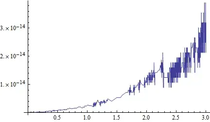
This looks pretty good to me.

Remarks

I went through all this because I wanted to reinforce the point I repeatedly am trying to make: Mathematica is many times more powerful when used as a tool we want to direct, rather than when one expects out of the box solutions for all problems - that won't happen.

Note that because we are able here to go quite a long way analytically, we have a much better insight and preparation for possible numerical implementation, for example when functions won't be so nice.