How to plot and solve the numerical solution of a integro-differential equation

Question

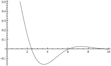
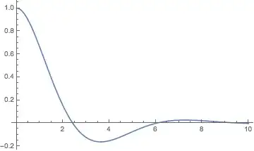
I have a integro-differential equation of the form $y'(t) = - \int_0^t {y(t_1 )} e^{t_1 - t} dt_1, {\rm{ t}} \in {\rm{[0,10], y(0) = 1}}$

My code is:

f[t_Real] := NIntegrate[y[t1]*Exp[t1-t], {t1, 0, t}];

solution1=NDSolve[{D[y[t], t]==-f[t], y[0] == 1}, y[t], {t, 0, 10}];

Plot[Evaluate[y[t] /. solution1], {t, 0, 10}, PlotRange -> All]

But this simply outputs the error:

NIntegrate::nlim: t1 = t is not a valid limit of integration.

Mathematica can't directly handle integro-differential equations. Try converting it to an ODE, before feeding it to NDSolve[]. — J. M.'s missing motivation, May 04 '13 at 04:20
I fixed some syntax errors in your code. Also I do not get the same error. I get NIntegrate::inumr (because of the symbolic y[t1] in the integral. You probably had a hidden definition f[t_] := NIntegrate[..] that you had not cleared. It's a good idea to restart the kernel and retry your code before posting. — Michael E2, Jun 01 '15 at 10:48

score 18 · Answer 1 · answered May 04 '13 at 04:48

18

This integral equation is solvable using the LaplaceTransform technique:

Clear[s, t];
eqn = y'[t] == -Integrate[y[t1] Exp[t1 - t], {t1, 0, t}]

LaplaceTransform[eqn, t, s]

(*
==> 
s LaplaceTransform[y[t], t, s] - y[0] == -(
  LaplaceTransform[y[t], t, s]/(1 + s))
*)

Solve[%, LaplaceTransform[y[t], t, s]]

(*
==> {{LaplaceTransform[y[t], t, s] -> ((1 + s) y[0])/(
   1 + s + s^2)}}
*)

InverseLaplaceTransform[%, s, t]

(*
==> {{y[t] -> (
   E^(-t/2) (Sqrt[3] Cos[(Sqrt[3] t)/2] + Sin[(Sqrt[3] t)/2]) y[0])/
   Sqrt[3]}}
*)

ySolution[t_] = y[t] /. First[%] /. y[0] -> 1

(*
==> (E^(-t/
  2) (Sqrt[3] Cos[(Sqrt[3] t)/2] + Sin[(Sqrt[3] t)/2]))/Sqrt[3]
*)

Plot[ySolution[t], {t, 0, 10}]

solution

answered May 04 '13 at 04:48

Jens

97,245
7
213
499

Thank you. But I need the numerical solution of the integro-differential equation. – user7260 May 04 '13 at 05:37
3

...@user, Jens gave you a closed form solution, which is a bit more useful. Why do you still need a numerical solution? Unless... what you posted is in fact not your actual problem. – J. M.'s missing motivation May 04 '13 at 06:23
Thank you very much! I want to compare the difference the numerical and exact solution of the integro-differential equation. – user7260 May 04 '13 at 07:15
@user7260 If you use this package for Laplace inversion, then you can get a semi-numerical solution. – xzczd Jun 07 '13 at 04:02

score 6 · Answer 2 · edited Apr 13 '17 at 12:55

This is probably what @Guess who it is. had in mind in the comment posted under the question.

solution1 = NDSolve[{
    D[y[t], t] == -Exp[-t] f0[t], y[0] == 1,
    f0'[t] == y[t]*Exp[t], f0[0] == 0},
   y[t], {t, 0, 10}];

Plot[Evaluate[y[t] /. solution1], {t, 0, 10}, PlotRange -> All]

Mathematica graphics

Comparison with Jens's exact solution and how well the combined PrecisionGoal/AccuracyGoal is satisfied:

jsol = (E^(-t/2) (Sqrt[3] Cos[(Sqrt[3] t)/2] + Sin[(Sqrt[3] t)/2])) / Sqrt[3];
Plot[Evaluate[{y[t] - jsol /. solution1,
      {1, -1} (10^-(MachinePrecision/2.) + 10^-(MachinePrecision/2.) jsol)} // Flatten],
 {t, 0, 10}]

Mathematica graphics

How to plot and solve the numerical solution of a integro-differential equation

2 Answers2

Linked

Related