3

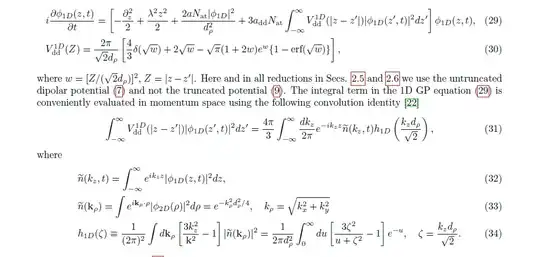
I am trying to solve numerically Equation number (29) with the help of Eq.(32) and (34) from this paper https://arxiv.org/pdf/1506.03283.pdf.

for

Subscript[N, at]=10000,a=100*Subscript[a, B]
Subscript[a, dd]=132.7*Subscript[a, B],Subscript[a, B]=5.29*10^-5,
Subscript[d, ρ]=1,λ=0.5

enter image description here

Subscript[a, dd] = 132.7*5.29*10^-5;
        a0 = 100*5.29*10^-5;
λ = 0.5;
n = 20;
xg = N[Range[n]]/(n + 1);
Subscript[d, ρ] = 1;
Nat = 10000
Subscript[h, 1 D] = 
 Interpolation[
  Table[{Subscript[k, z], 
    NIntegrate[
     1/(2 π (Subscript[d, ρ])^2) ((
        3 ((Subscript[k, z] Subscript[d, ρ])/Sqrt[2])^2)/(
        u + ((Subscript[k, z] Subscript[d, ρ])/Sqrt[2])^2) - 
        1) Exp[-u], {u, 0, ∞}]}, {Subscript[k, z], 1, 2, 
    0.005}]]
uxx[u_?VectorQ] := Module[{n = Length[u]},
  FourierDST[Subscript[h, 1 D] FourierDST[u, 1], 1]]
usol = NDSolveValue[{I D[ϕ[z, t], 
      t] = -1/2 D[ϕ[z, t], z, z] + 
      1/2 λ^2 z^2 ϕ[z, t] + (
       2 a Nat)/(Subscript[d, ρ])^2 Abs[ϕ[z, t]]^2 ϕ[z,
         t] + 3 Subscript[a, dd]  Subscript[N, at]
        uxx[ϕ[z, t]] ϕ[z, t] == 0, ϕ[z, 0] == 
    E^(-λ (xg)^2/2)*(λ/Pi)^(1/4), ϕ[n, 
     t] = ϕ[-n, t]}, ϕ, {t, 0, 20}, {z, -n, n}]
Plot3D[Abs[usol[z,t]]^2, {t, 0, 1}, {z, -a/1.5, 0}, PlotPoints -> 50,
  ColorFunction -> "Rainbow"]

This code is able to find the ground state of the equation without the Last Integral Term

m = ℏ = 1;
λ = 0.5;
L = 10;
aB = 5.29*10^-5;
a0 = 100*aB;
dρ = 1;
add = 132.7*aB;
Nat = 10000;
nmax = 1000;
Δ = L/(nmax + 1);
zgrid = Range[nmax]*Δ;
W[z_] = λ*z^2/2;
Wgrid = W /@ zgrid;
groundstate[δβ_?NumericQ, κ_?NumericQ, 
   tolerance_: 10^-10] := 
  Module[{Ke, propKin, propPot2, prop, v0, ϕ},
   (* compute the diagonal elements of exp[-δβ*T] *)
   Ke = Exp[-δβ*Range[nmax]^2*(π^2 ℏ^2)/(
       2 m L^2)] // N;
   (* propagate by a full imaginary-time-step with T *)
   propKin[v_] := Normalize[FourierDST[Ke*FourierDST[v, 1], 1]];
   (* propagate by a half imaginary-time-step with V *)
   propPot2[v_] := 
    Normalize[
     Exp[-(δβ/
         2)*(Wgrid + κ*Abs[v]^2/Δ)]*v];
   (* propagate by a full imaginary-time-step by *)
   (* H=T+V using the Trotter approximation *)
   prop[v_] := propPot2[propKin[propPot2[v]]];
   (* random starting point *)
   v0 = Normalize@RandomVariate[NormalDistribution[], nmax];
   (* propagation to the ground state *)
   ϕ = 
    FixedPoint[prop, v0, 
     SameTest -> Function[{v1, v2}, Norm[v1 - v2] < tolerance]];
   {ϕ}];
With[{κ = (2*a0*Nat)/(dρ)^2, δβ = 10^-4},
 {ϕ} = groundstate[δβ, κ];
 ListLinePlot[
  Join[{{0, 0}}, {zgrid, 
     Abs[ϕ]^2/Δ}\[Transpose], {{L, 0}}], 
  PlotRange -> All]]

I tried to include the last term in the module but failed. If Anyone can help me with this...

h1D = Interpolation[
  Table[{kz, 
    NIntegrate[
     1/(2 π (dρ)^2) ((3 ((kz dρ)/Sqrt[2])^2)/(
        u + ((kz dρ)/Sqrt[2])^2) - 1) Exp[-u], {u, 
      0, ∞}]}, {kz, 1, 2, 0.005}]]
FourierDST[h1D FourierDST[v, 1], 1]]
xzczd
  • 65,995
  • 9
  • 163
  • 468
Argha Debnath
  • 311
  • 2
  • 11
  • 3
    You may get helpful responses if you share what you have already tried. – Michael Stern Mar 30 '22 at 11:43
  • Get familiar with the Mathematica solvers NDSolve and NDSolveValue. Start small. Review the examples. Type NDSolve, hover over it, press the "I" and work through the examples. Do simple ones first, take some time, then attempt to code yours. Cut and paste your code for others to review. – josh Mar 30 '22 at 12:53
  • Do you need Mathematica code for this model? Please, note, that Fortran and CUDA version have been upload on http://cpc.cs.qub.ac.uk/summaries/AEWL_v1_0.html – Alex Trounev Mar 30 '22 at 15:25
  • @AlexTrounev Resected sir, I have checked that already but I am eager to solve in MATHEMATICA using split-step Crank-Nicolson Method. – Argha Debnath Mar 31 '22 at 08:26
  • @AlexTrounev I am unable to add the last integral term in the equation. Looking forward for your suggestions. – Argha Debnath Apr 06 '22 at 10:00
  • @ArghaDebnath Please, see my answer. – Alex Trounev Apr 07 '22 at 10:33

1 Answers1

6

We can use GaussianQuadratureWeights[] to compute integrals as in Fortran code in the paper cited. On the first step we define initial data as follows

Needs["NumericalDifferentialEquationAnalysis`"];

np = 81; g = GaussianQuadratureWeights[np, -L, L]; points = g[[All, 1]]; weights = g[[All, 2]];

sol[0][z_, t_] := E^(-[Lambda] (z)^2/2)([Lambda]/Pi)^(1/4); a0 = 5.2910^-5; a = 113 a0; dp = 1; add = 132.75.2910^-5; Nat = 100; L = 10; [Lambda] = 0.5; dt = 1/100; nt = 600; T = Table[i dt, {i, 0, 1001}];

h1[x_?NumericQ] := 1/(2 Pi dp^2) NIntegrate[ Exp[-u] (3 x^2/(u + x^2) - 1), {u, 0, Infinity}]; h1D = Table[h1[x dp/Sqrt[2]], {x, points}];

nk[0] = Table[ Sum[weights[[i]] Exp[ I points[[j]] points[[i]]] Abs[sol[0][points[[i]], 0]]^2, {i, Length[g]}], {j, Length[g]}]; intn[0] = 2/3 Table[{points[[j]], Re[Sum[weights[[i]] Exp[-I points[[j]] points[[i]]] h1D[[ i]] nk[0][[i]], {i, Length[g]}]]}, {j, Length[g]}]; Vdd[0] = Interpolation[ Join[{{-L, intn[0][[1, 2]]}}, intn[0], {{L, intn[0][[np, 2]]}}]];

Then we organize loop to compute solution on every step. There are two possible solutions. To compute nonstationary state we use real time computation as follows

Do[sol[s] = 
   NDSolveValue[{-I D[\[Phi][z, t], t] - 1/2 D[\[Phi][z, t], z, z] + 
        1/2 \[Lambda]^2 z^2 \[Phi][z, 
          t] + (2 a Nat)/(dp)^2 Abs[\[Phi][z, t]]^2 \[Phi][z, t] + 
        3 add Nat Vdd[s - 1][z] \[Phi][z, t] == 0, \[Phi][z, T[[s]]] ==
        sol[s - 1][z, T[[s]]], \[Phi][L, t] == 0, \[Phi][-L, t] == 
       0}, \[Phi], {t, T[[s]], T[[s + 1]]}, {z, -L, L}, 
     Method -> {"MethodOfLines", 
       "SpatialDiscretization" -> {"TensorProductGrid", 
         "MinPoints" -> 40, "MaxPoints" -> np, 
         "DifferenceOrder" -> "Pseudospectral"}}] // Quiet; 
  nk[s] = Table[
    Sum[weights[[i]] Exp[
       I points[[j]] points[[i]]] Abs[
        sol[s][points[[i]], T[[s + 1]]]]^2, {i, Length[g]}], {j, 
     Length[g]}];
  intn[s] = 
   2/3 Table[{points[[j]], 
      Re[Sum[weights[[i]] Exp[-I points[[j]] points[[i]]] h1D[[
          i]] nk[s][[i]], {i, Length[g]}]]}, {j, Length[g]}];
  Vdd[s] = 
   Interpolation[
    Join[{{-L, intn[s][[1, 2]]}}, 
     intn[s], {{L, intn[s][[np, 2]]}}]];, {s, 1, 
   nt}]

Visualization of the integral term and numerical solution

Table[Plot[Vdd[s][z], {z, -L, L}, Frame -> True, 
  PlotLabel -> 1. dt s], {s, 0, nt,30}] 

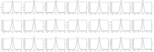
Figure 1

Table[Plot[Abs[sol[s][z, T[[s + 1]]]], {z, -L, L}, Frame -> True, 
  PlotLabel -> 1. dt s, PlotRange -> All], {s, 0, nt, 30}]

Figure 2

To compute rms size $<z>$ we use

rms = Table[{s, 
   Re[NIntegrate[
      z^2 sol[s][z, T[[s + 1]]] Conjugate[
        sol[s][z, T[[s + 1]]]], {z, -L, L}, PrecisionGoal -> 4, 
      AccuracyGoal -> 5]]^.5}, {s, 1, nt}]

Visualization

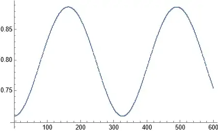
ListPlot[rms]

Figure 3

This is not stationary state nevertheless for about one period we have

meanr = 
 Mean[Take[rms], 328]] // Last

(Out[]= 0.798857)

In the Table 1 this value is about 0.7939 (variational method) or 0.7937 (imaginary time method).To compute ground state we use imaginary time method

Do[sol1[s] = 
   NDSolveValue[{ 
      D[\[Phi][z, t], t] - 1/2 D[\[Phi][z, t], z, z] + 
        1/2 \[Lambda]^2 z^2 \[Phi][z, 
          t] + (2 a Nat)/(dp)^2 Abs[\[Phi][z, t]]^2 \[Phi][z, t] + 
        3 add Nat Vdd[s - 1][z] \[Phi][z, t] == 0, \[Phi][z, T[[s]]] ==
        sol[s - 1][z, T[[s]]], \[Phi][L, t] == 0, \[Phi][-L, t] == 
       0}, \[Phi], {t, T[[s]], T[[s + 1]]}, {z, -L, L}, 
     Method -> {"MethodOfLines", 
       "SpatialDiscretization" -> {"TensorProductGrid", 
         "MinPoints" -> 40, "MaxPoints" -> np, 
         "DifferenceOrder" -> "Pseudospectral"}}] // Quiet; 
  nk[s] = Table[
    Sum[weights[[i]] Exp[
       I points[[j]] points[[i]]] Abs[
        sol[s][points[[i]], T[[s + 1]]]]^2, {i, Length[g]}], {j, 
     Length[g]}];
  intn[s] = 
   2/3 Table[{points[[j]], 
      Re[Sum[weights[[i]] Exp[-I points[[j]] points[[i]]] h1D[[
          i]] nk[s][[i]], {i, Length[g]}]]}, {j, Length[g]}];
  Vdd[s] = 
   Interpolation[
    Join[{{-L, intn[s][[1, 2]]}}, 
     intn[s], {{L, intn[s][[np, 2]]}}]];, {s, 1, 
   nt}] 

To compute rms size $<z>$ we use

rmsg = Table[{s, 
   Re[NIntegrate[
      z^2 sol1[s][z, T[[s + 1]]] Conjugate[
        sol1[s][z, T[[s + 1]]]], {z, -L, L}, PrecisionGoal -> 4, 
      AccuracyGoal -> 5]]^.5}, {s, 1, nt}]

Mean value in one period is about

Mean[Take[rmsg, 328]] // Last

Out[]= 0.791021

Alex Trounev
  • 44,369
  • 3
  • 48
  • 106
  • @AexTrounev Thanks for the solution and giving a great deal of importance to my problem. I like to ask how can I get stationary or ground state solution from this as I need them to calculate Energy and chemical potential. Also dynamical evaluation of the density wave. If you can recommend me advance tutorial or books in MATHEMATICA so that I can deal with typical nonlinear equation or coupled nonlinear equations. I already studied some of your previous solutions. They are helping me immensely. – Argha Debnath Apr 13 '22 at 05:08
  • @ArghaDebnath Please, see update to my answer. – Alex Trounev Apr 13 '22 at 14:24
  • Thanks for quick response and also for the solutions. @AlexTrounev – Argha Debnath Apr 14 '22 at 09:40