Numerical solution of the inverse contour plot

Question

I have a function $f(u,v)$ on some domain of $(u,v)$ and would like to find (numerically) the set of couples* $(u_0,v_0)$ s.t. $f(u_0,v_0)=0$, for instance (just and example to illustrate, in practice I will use arbitrary non analytical functions)

  ContourPlot[BesselJ[3, Sin[u^2 - v]] == 0, {u, -1, 1}, {v, -1, 1}]

FindRoot does not work immediately because it needs two equations. Any easy implementation for this problem ?

*"the set of couples" has naturally infinite elements, so I would expect a set of finitely countable elements with adjustable density.

Answer 1

The problem appears to be solvable with an exact approach, e.g.

Reduce[ BesselJ[3, Sin[u^2 - v]] == 0 && 
        -1 <= u <= 1 && -1 <= v <= 1, {u, v}]

  -1 <= u <= 1 && v == u^2

Nevertheless numerically one can solve it this way:

sol[u_] = v /. NSolve[ BesselJ[3, Sin[u^2 - v]] == 0 &&
                      -1 <= u <= 1 && -1 <= v <= 1, {u, v}] //First//Quiet;

or with FindRoot (this is more powerful when we deal with special functions):

ns[u_] := v /. FindRoot[BesselJ[3, Sin[u^2 - v]] == 0, {v, 0}]
{sol[0.37], ns[0.37]}

 {0.1369, 0.1369}

In case of a more involved equations we could modify starting point in FindRoot or exploit various options e.g. First positive root.

Plot[{sol[u], ns[u]}, {u, -1, 1}, PlotStyle -> {Blue, Dashed}]

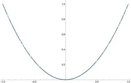
If a set of pairs $(u,v)$ is needed, let's go a directly taking $100$ random arguments:

dmn = RandomReal[{-1, 1}, 100];
SetAttributes[ns, Listable]
pairs = Transpose[{dmn, ns[dmn]}];
ListPlot[Transpose[{dmn, ns[dmn]}]]

Answer 2

sol = FindInstance[{BesselJ[3, Sin[u^2 - v]] == 0, -1 <= u <= 1, -1 <=
      v <= 1}, {u, v}, 1000];
ListPlot[{u, v} /. sol]

Replay to comment

Clear[sol, pts]; sol = 
 FindInstance[{BesselJ[3, Sin[u^2 - v]] == 0, -1 <= u <= 1, -1 <= v <=
     1}, {u, v}, 1000];
pts = SortBy[{u, v} /. sol, First];
Plot[Interpolation[pts][x], {x, -1, 1}]

Answer 3

Take the point pairs from ContourPlot

pic = ContourPlot[BesselJ[3, Sin[u^2 - v]] == 0,{u, -1, 1}, {v, -1, 1}]
uvi= pic[[1]][[1, 1]];
Show[pic, ListPlot[uvi, PlotStyle -> Red]]

If necessary you might take these values as starting point for further improvement with FindRoot

uviI = Map[{#[[1]], v} /.FindRoot[BesselJ[3, Sin[#[[1]]^2 - v]] ==0, {v, #[[2]]}] &, uvi];
Show[pic,ListPlot[{uvi, uviI, uviI}, PlotStyle ->{Red, Blue, Cyan}, Joined -> {False, False, True}]]

Answer 4

Clear["Global`*"]

To use FindRoot directly,

vSol[u_?NumericQ, est_ : 1/2] :=
 v /. FindRoot[BesselJ[3, Sin[u^2 - v]] == 0, {v, est}]
Plot[vSol[u], {u, -1, 1},
 Frame -> True,
 FrameLabel -> (Style[#, 14, Bold] & /@ {u, v})]

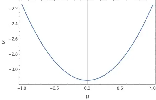
Change the initial estimate of the root to get a different branch.

Plot[vSol[u, 1/2 - Pi], {u, -1, 1},
 Frame -> True,
 FrameLabel -> (Style[#, 14, Bold] & /@ {u, v})]

Answer 5

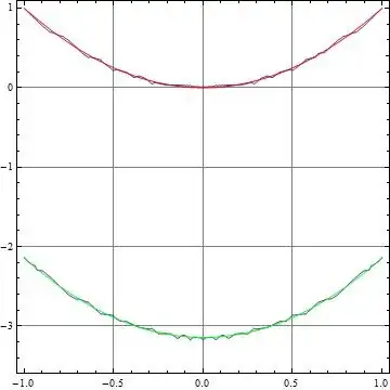
Regard v as function of u, v[u], and differentiate function f[u,v[u]] to be zero with respect to u and generate interpolating function for v[u] with NDSolve.

Here shown for two branches.

f[u_, v_] = BesselJ[3, Sin[u^2 - v]];
cp = ContourPlot[f[u, v] == 0, {u, -1, 1}, {v, -3.5, 1}];
fi1 = First@
  FindInstance[f[u, v] == 0 && -1 < u < 1 && -1 < v < 1, {u, v}]
fi2 = First@
  FindInstance[f[u, v] == 0 && -1 < u < 1 && -3 < v < -2, {u, v}]
vsol1 = v /. 
   First@NDSolve[{D[f[u, v[u]], u] == 0, v[u /. fi1] == (v /. fi1)}, 
     v, {u, -1, 1}];
vsol2 = v /. 
   First@NDSolve[{D[f[u, v[u]], u] == 0, v[u /. fi2] == (v /. fi2)}, 
     v, {u, -1, 1}];
pl = Plot[{vsol1[u], vsol2[u]}, {u, -1, 1}, PlotStyle -> {Red, Green}];
Show[cp, pl, GridLines -> Automatic, Frame -> True]