ListDensityPlot performance when scaling axes

Question

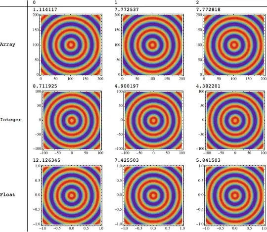
I need to visualize 3D data having 200*200 data points. ListDensityPlot is a good candidate, but it seems to have strange performance issues. I created a small test that plots 40000 points. It has three cases: using 2D array as input, using array of 3D points with integer coordinates $(x,y)$ and using array of 3D points with float coordinates $(x,y)$.

    TestFunction[x_, y_] := Sin[Pi/20* Sqrt[x^2 + y^2]];
    testdata = Table[TestFunction[i, j], {i, -100, 100}, {j, -100, 100}];
    testdataPoints = 
      Flatten[Table[{i, j, TestFunction[i, j]}, {i, -100, 100}, {j, -100, 
         100}], 1];
    testdataPoints2 = 
      Flatten[Table[{i*0.01, j*0.01, TestFunction[i, j]}, {i, -100, 
         100}, {j, -100, 100}], 1];
Benchmark[d_, n_] := 
  Timing[ListDensityPlot[d, ColorFunction -> "Rainbow", 
    PlotRange -> Full, InterpolationOrder -> n]];
TableForm[
 Table[Benchmark[data, 
   n], {data, {testdata, testdataPoints, testdataPoints2}}, {n, 0, 
   2}], TableHeadings -> {{"Array", "Integer", "Float"}, {0, 1, 2}}]

density plots of different data

It gives pretty strange result. When I simply scale axes and my coordinates are not integer anymore (the case is called "Float"). The performance drops almost 10 times (3 seconds vs 25 seconds).

Here's the output timing:

            0         1         2
Array   0.834276 2.96802    3.05685  
Integer 4.84968  3.42562    3.19835
Float   27.5574   26.1669   25.9262

Any explanation for such behavior?

Edit

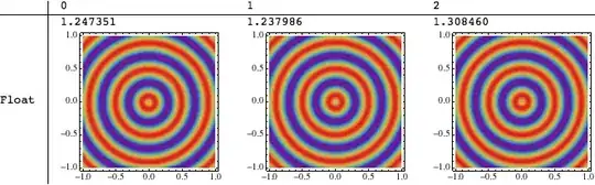
As alternative to Michael's solution one can use ArrayPlot (as Silvia suggested) if interpolation is not important. It can be easily scaled to look like "Float" case.

"I can't post image" - can you post it somewhere else, like imgur, and then link to the image in your post? — J. M.'s missing motivation, Jun 18 '13 at 15:00
I don't think image really matters, but you can easily run the test code. The generated images are identical (as my eye sees that). It's timing that puzzles me — BlacKow, Jun 18 '13 at 15:04
Anyway... what is the result of applying Developer`PackedArrayQ[] on your three lists? — J. M.'s missing motivation, Jun 18 '13 at 15:15
Developer`PackedArrayQ /@ {testdata, testdataPoints, testdataPoints2} gives {False, False, False}. — BlacKow, Jun 18 '13 at 15:19
By the way, using Interpolation, DensityPlot and PlotPoints -> 101 is faster for me than ListDensityPlot. (Not an answer to your Q, though.) — Michael E2, Jun 18 '13 at 15:20
Well, can you do another set of tests, with packed versions of your lists? (e.g. packedtestdata = Developer`ToPackedArray[testdata]). — J. M.'s missing motivation, Jun 18 '13 at 15:21
@0x4A4D He needs to N to the data first: Developer`ToPackedArray[N[testdata]]. — Michael E2, Jun 18 '13 at 15:24
This is probably because the Delaunay triangulation used by ListDensityPlot is very inefficient. See this Q&A for some details. — rm -rf, Jun 18 '13 at 15:25
@Michael E2 packedtestdata = Developer``ToPackedArray /@ {N[testdata], N[testdataPoints], N[testdataPoints2]}; Gives same result, maybe a fraction of second less — BlacKow, Jun 18 '13 at 15:33
@rm-rf how is triangulation more effective for integer (x,y)? — BlacKow, Jun 18 '13 at 15:35
@BlacKow You need to use double back-ticks to wrap a inline code which contains back-tick. — Silvia, Jun 18 '13 at 15:39
@BlacKow Sorry, but I'm not a triangulation expert, so I don't know the answer to that (or if that indeed is the reason). All I know is that the built-in Delaunay triangulation is inefficient for all but small 2D lists... 0x4A4D or Szabolcs or halirutan might be able to shed more light on it, if they happen to see this question. — rm -rf, Jun 18 '13 at 15:40
You can always use the poor man's ListDensityPlot, that is the ArrayPlot. — Silvia, Jun 18 '13 at 15:59
@Silvia Yes, I can, but then I need to deal with labeling the axes with FrameTicks which is an additional effort — BlacKow, Jun 18 '13 at 16:29

score 5 · Accepted Answer · edited Apr 13 '17 at 12:56

5

Too long for a comment:

Packing the data, as @0x4A4D suggests, seems to "fix" the problem, except in InterpolationOrder -> 0. See What is a Mathematica packed array? for an explanation of the importance of packed arrays.

TableForm[
 ParallelTable[
  Benchmark[data, n],
  {data,  Developer`ToPackedArray /@ N@{testdata, testdataPoints, testdataPoints2}},
  {n, 0, 2}], 
 TableHeadings -> {{"Array", "Integer", "Float"}, {0, 1, 2}}]

Table of output

This way is faster:

TableForm[
 Table[
  Timing[
   ifn = Interpolation[data, InterpolationOrder -> n]; 
   DensityPlot[ifn[i, j],
    {i, -1, 1}, {j, -1, 1}, PlotPoints -> 101, 
    ColorFunction -> "Rainbow", PlotRange -> Full]],
  {data, {testdataPoints2}}, {n, 0, 2}], 
 TableHeadings -> {{"Float"}, {0, 1, 2}}]

Second table output

edited Apr 13 '17 at 12:56

Community

1

answered Jun 18 '13 at 15:47

Michael E2

235,386
17
334
747

Your last code need about 39, 40, 37 seconds for each InterpolationOrder settings respectively, while OP's code needs 46, 36, 35 seconds. Well I guess I really should upgrade my computer... – Silvia Jun 18 '13 at 15:57
@Silvia I'm on an 2.7GHz i7 Mac, 16GB RAM. – Michael E2 Jun 18 '13 at 16:00
In my case - OS X, Mathematica 8 - the packing gives: 16.9, 13.9, 13.7 for "Float" case, so its twice faster but it is still significantly slower than "Integer" case, which is really bizarre. – BlacKow Jun 18 '13 at 16:02
The last code gives 0.84, 0.82, 0.88, so its's a nice workaround. Thanks! – BlacKow Jun 18 '13 at 16:03
I'm using a core 2 quad CPU @2.4GHz and 8G RAM. So it seems not quite natural to take such a long time on my PC? – Silvia Jun 18 '13 at 16:08

ListDensityPlot performance when scaling axes

Edit

1 Answers1

Linked