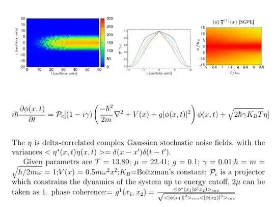
Solving Stochastic Gross-Pitaevskii equation

Question

I am trying to solve the Stochastic Gross-Pitaevskii equation from this paper https://arxiv.org/pdf/1409.0146.pdf. But I have no idea how to solve adding a noise term. I like to see the wave function after adding a temperature similar to https://arxiv.org/pdf/2107.06680.pdf fig(1). Below is the problem statement from https://arxiv.org/pdf/1409.0146.pdf and the results I want to see.

 ClearAll["Global`*"]
xtab = Table[i/10, {i, 1, 300}];
ttab = Table[i/10, {i, 1, 301}];

Noisetab = Table[Random[Real, {-1/5, 1/5}], {301}];

\[Eta] = Interpolation[
   Join[Table[{-xtab[[i]], ttab[[i]], Noisetab[[i]]}, {i, 300}], 
    Table[{0, ttab[[i]], Noisetab[[i]]}, {i, 300}], 
    Table[{xtab[[i]], ttab[[i]], Noisetab[[i]]}, {i, 300}]]];

hbar = 1; mass = 1;
\[Gamma] = 0.01; g = 0.1; temp = 13.89; \[Mu] = 22.41; \[Omega] = 0.5;
\[Epsilon] = 1 - I*\[Gamma]; kb = 1;

pse[x_, t_] := Exp[-0.2 x^2];
sol = NDSolveValue[{ - 
      D[u[x, t], t] == -0.5 \[Epsilon] D[u[x, t], {x, 2}] + 
      0.5 \[Epsilon] \[Omega]^2 x^2 u[x, 
        t] + \[Epsilon] g Abs[u[x, t]]^2 u[x, t] - \[Epsilon] \[Mu] u[
        x, t] + Sqrt[2  \[Gamma] kb temp] \[Eta][x, t], u[x, 0] == 0, 
    u[30, t] == 0, u[-30, t] == 0},
   u, {x, -30, 30}, {t, 0, 20}, 
   Method -&gt; {&quot;MethodOfLines&quot;, 
     &quot;SpatialDiscretization&quot; -&gt; {&quot;TensorProductGrid&quot;, 
       &quot;MinPoints&quot; -&gt; 161, &quot;MaxPoints&quot; -&gt; 201, 
       &quot;DifferenceOrder&quot; -&gt; 4}}, MaxSteps -&gt; 10^6];

DensityPlot[Abs[sol[x, t]]^2, {t, 0, 20}, {x, -30, 30}, 
 AspectRatio -&gt; 1/2, Frame -&gt; True, FrameTicks -&gt; Automatic, 
 PlotPoints -&gt; 200, ImageSize -&gt; 1000, 
 LabelStyle -&gt; {24, Bold, Large, Black}, 
 ColorFunction -&gt; &quot;BlueGreenYellow&quot;, 
 FrameLabel -&gt; {{Style[&quot;x&quot;, FontFamily -&gt; &quot;Times New Roman&quot;, 
     FontSlant -&gt; &quot;Italic&quot;, FontWeight -&gt; Bold, FontSize -&gt; 30], 
    None}, {Style[&quot;t&quot;, FontFamily -&gt; &quot;Times New Roman&quot;, 
     FontSlant -&gt; &quot;Italic&quot;, FontWeight -&gt; Bold, FontSize -&gt; 30], 
    None}}]

I tried pseudospectral Method

ClearAll["Global`*"]
xtab = Table[i/10, {i, 1, 800}];
ttab = Table[i/10, {i, 1, 801}];
Noisetab = Table[Random[Real, {-1/5, 1/5}], {801}];
[Eta] = Interpolation[
   Join[Table[{-xtab[[i]], ttab[[i]], Noisetab[[i]]}, {i, 800}], 
    Table[{0, ttab[[i]], Noisetab[[i]]}, {i, 800}], 
    Table[{xtab[[i]], ttab[[i]], Noisetab[[i]]}, {i, 800}]]];
hbar = 1; mass = 1;
[Gamma] = 0.01; g = 0.1; temp = 13.89; [Mu] = 22.41; [Omega] = 0.5;
[Epsilon] = 1 - I*[Gamma]; kb = 1;
pse[x_, t_] := Exp[-0.2 x^2];
sol = NDSolveValue[{ 
    I D[u[x, t], t] == -0.5 [Epsilon] D[u[x, t], {x, 2}] + 
      0.5 [Epsilon] [Omega]^2 x^2 u[x, 
        t] + [Epsilon] g Abs[u[x, t]]^2 u[x, t] - [Epsilon] [Mu] u[
        x, t] + Sqrt[2  [Gamma] kb temp] [Eta][x, t], u[x, 0] == 0, 
    u[30, t] == 0, u[-30, t] == 0},
   u, {x, -30, 30}, {t, 0, 80}, 
   Method -> {"MethodOfLines", 
     "SpatialDiscretization" -> {"TensorProductGrid", 
       "MinPoints" -> 100, "MaxPoints" -> 161, 
       "DifferenceOrder" -> "Pseudospectral"}}, MaxSteps -> 10^6];
DensityPlot[Abs[sol[x, t]]^2, {t, 0, 80}, {x, -30, 30}, 
 AspectRatio -> 1/2, Frame -> True, FrameTicks -> Automatic, 
 PlotPoints -> 200, ImageSize -> 1000, 
 LabelStyle -> {24, Bold, Large, Black}, 
 ColorFunction -> "BlueGreenYellow", 
 FrameLabel -> {{Style["x", FontFamily -> "Times New Roman", 
     FontSlant -> "Italic", FontWeight -> Bold, FontSize -> 30], 
    None}, {Style["t", FontFamily -> "Times New Roman", 
     FontSlant -> "Italic", FontWeight -> Bold, FontSize -> 30], 
    None}}]

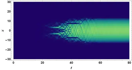
The result looks like

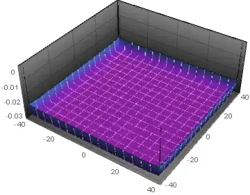
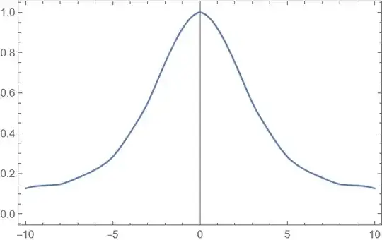
Can anyone help me with phase coherence g(x_1,x_2) and its dynamics? Also how to get a ground-state solution like https://arxiv.org/pdf/2107.06680.pdf with the inclusion of temperature? I tried with 2D equation from Solving logarithmic 2D Nonlinear GPE Equation.

ClearAll["Global`*"]
\[Gamma] = 0.01; g = 0.1; temp = 13.89; \[Mu] = 22.41; \[Omega] = 0.02;
\[Epsilon] = 1 - I*\[Gamma]; kb = 1;
data = Flatten[
   Table[{{x, y, t}, Random[Real, {-1/100, 1/100}]}, {x, -40, 
     40}, {y, -40, 40}, {t, 0, 10}], 2];
[Eta] = Interpolation[data, InterpolationOrder -> 1];
boundary = 40; xl = yl = -boundary; xr = yr = boundary;
finalt = 10;
seedwave[x_, y_] := 
  Exp[-0.05 (x^2 + y^2) + 
     Isvalue ArcTan[x, y]] (x^2 + y^2)^(svalue/2);
pnumber = 
  NIntegrate[
   Exp[-0.05 (x^2 + 
       y^2)], {x, -[Infinity], [Infinity]}, {y, -[Infinity], 

[Infinity]}];(particle number check*)
svalue = 0; lvalue = 0;
sol = NDSolveValue[{-D[[Psi][x, y, t], 
      t] == -0.5 [Epsilon] Laplacian[[Psi][x, y, t], {x, 
        y}] + [Epsilon] Abs[[Psi][x, y, t]]^2 [Psi][x, y, t] Log[
       Abs[[Psi][x, y, t]]^2] - [Epsilon] [Mu] [Psi][x, y, t] + 
     Sqrt[2  [Gamma] kb temp] [Eta][x, y, t], [Psi][xl, y, t] == 
    0, [Psi][xr, y, t] == 0, [Psi][x, yl, t] == 
    0, [Psi][x, yr, t] == 0, [Psi][x, y, 0] == 0.1}, [Psi][x, y, 
   t], {x, xl, xr}, {y, yl, yr}, {t, 0, finalt}, 
  Method -> {"MethodOfLines", 
    "SpatialDiscretization" -> {"TensorProductGrid", 
      "MinPoints" -> 40, "MaxPoints" -> 81, 
      "DifferenceOrder" -> "Pseudospectral"}}, MaxSteps -> 10^6]
Plot3D[Evaluate[Abs[sol]^2 /. t -> finalt], {x, xl, xr}, {y, yl, yr}, 
 PlotRange -> All, MeshStyle -> White, ColorFunction -> "Rainbow", 
 PlotTheme -> "Marketing", PlotPoints -> 100]

And the phase

Plot3D[Evaluate[Arg[sol] /. t -> finalt], {x, xl, xr}, {y, yl, yr}, 
 PlotRange -> All, MeshStyle -> White, ColorFunction -> "Rainbow", 
 PlotTheme -> "Marketing", PlotPoints -> 100]

What's wrong with the error message you get? That needs to be fixed first. — user21, Nov 03 '22 at 10:28
Due to the stochastic term, you might need to use ItoProcess instead of NDSolve, which would entail manually discretizing your equation in space. Here's an example applied to a stochastic reaction-diffusion equation. — Chris K, Nov 03 '22 at 13:28
@ArghaDebnath I see you've edited your question to use ItoProcess now. Did it work or are you still having problems? — Chris K, Nov 04 '22 at 13:02
@ArghaDebnath I suggest adding that info to your question so that others can see that a problem remains. — Chris K, Nov 04 '22 at 17:20
I like to know @Chris K in https://mathematica.stackexchange.com/questions/23183/itoprocess-for-stochastic-reaction-diffusion-equation/ if it was N[x,y,t], then how would someone define w and n ? — Argha Debnath, Nov 05 '22 at 06:24
@ArghaDebnath Please pay attention what they did in a paper cited: "We use 10 000 realizations to reduce noise in the density correlations". — Alex Trounev, Nov 18 '22 at 04:32
So, @AlexTrounev if it was just one realization then how to find a correlation and how can I use Pc, the projection operator? For this kind of case is my process alright or ItoProcess needed? In Pseudospectral Method, I have to give the initial condition as \psi[x,0]=0, otherwise, it is not working. — Argha Debnath, Nov 18 '22 at 05:18
In the 2D case, I started with the number 0.1 as my initial wave. — Argha Debnath, Nov 18 '22 at 05:26
@ArghaDebnath Ok, for one run we can compute correlation with using mean in time. — Alex Trounev, Nov 18 '22 at 06:07

Alex Trounev · Accepted Answer · 2022-11-21T03:50:19.547

We can compute correlation function with OrnsteinUhlenbeckProcess[] using mean in time as follows

tmax = 60; xmax = 60; nmax = 240;
pR = RandomFunction[
  OrnsteinUhlenbeckProcess[0, 1., xmax/nmax/Sqrt[2]], {0, xmax, 
   xmax/nmax}]; pI = 
 RandomFunction[
  OrnsteinUhlenbeckProcess[0, 1., xmax/nmax/Sqrt[2]], {0, xmax, 
   xmax/nmax}];
xR = Interpolation[pR, InterpolationOrder -> 1]; xI = 
 Interpolation[pI, InterpolationOrder -> 1];
eta[x_] = xR[x] + I xI[x];
tR = RandomFunction[
  OrnsteinUhlenbeckProcess[0, 1., tmax/nmax/Sqrt[2]], {0, tmax, 
   tmax/nmax}]; tI = 
 RandomFunction[
  OrnsteinUhlenbeckProcess[0, 1., tmax/nmax/Sqrt[2]], {0, tmax, 
   tmax/nmax}];
etR = Interpolation[tR, InterpolationOrder -> 1]; etI = 
 Interpolation[tI, InterpolationOrder -> 1];
eta1[t_] = etR[t] + I etI[t];

Solution

hbar = 1; mass = 1;
\[Gamma] = 0.01; g = 0.1; temp = 13.89; \[Mu] = 22.41; \[Omega] = \
0.5;
\[Epsilon] = 1 - I*\[Gamma]; kb = 1;
sol = NDSolveValue[{I D[u[x, t], 
        t] == -0.5 \[Epsilon] D[u[x, t], {x, 2}] + 
       0.5 \[Epsilon] \[Omega]^2 x^2 u[x, 
         t] + \[Epsilon] g Abs[u[x, t]]^2 u[x, 
         t] - \[Epsilon] \[Mu] u[x, t] + 
       Sqrt[2 \[Gamma] kb temp] eta[x + xmax/2] eta1[t]/4, 
     u[x, 0] == 0, u[xmax/2, t] == 0, u[-xmax/2, t] == 0}, 
    u, {x, -xmax/2, xmax/2}, {t, 0, tmax}, 
    Method -> {"MethodOfLines", 
      "SpatialDiscretization" -> {"TensorProductGrid", 
        "MinPoints" -> 141, "MaxPoints" -> nmax, 
        "DifferenceOrder" -> 4}}, MaxSteps -> 10^6] // Quiet;

Visualization

DensityPlot[Abs[sol[x, t]]^2, {t, 0, tmax}, {x, -20, 20}, 
 AspectRatio -> Automatic, PlotPoints -> 100, 
 ColorFunction -> "LightTemperatureMap", FrameLabel -> {"t", "x"}, 
 PlotRange -> All, PlotLegends -> Automatic]

Correlation function

phi[x_] = Sum[sol[x, t], {t, tmax - 20, tmax, 1/5}]/100; 
int[x_, x1_] = 
 Conjugate[phi[x1]] phi[x1 + x]/
   Sqrt[Abs[phi[x1]]^2 Abs[phi[x1 + x]]^2];
gbar1[x_?NumericQ] := 
  1/20 NIntegrate[Evaluate[int[x, x1]], {x1, -10, 10}, 
    Method -> "MonteCarlo", AccuracyGoal -> 2, PrecisionGoal -> 2];
lst1 = Table[{x, Re[gbar1[x]] // Quiet}, {x, -10, 10, 1}];
cor = Interpolation[lst1];

Visualization

Plot[.5 (cor[x] + cor[-x]), {x, -10, 10}]

Note, it is not zero at $x=\pm 10$, probably we need accumulate more data.

Thanks, @AlexTrounev. I will try it in 2D to see If I can get results like https://arxiv.org/pdf/2107.06680.pdf posted above fig (c). — Argha Debnath, Nov 18 '22 at 07:17
Ok, I have to increase the grid points to see the variations. — Argha Debnath, Nov 20 '22 at 12:32
@ArghaDebnath Use xmax=60 and plot in the range {x,-20, 20}. Code has been updated. — Alex Trounev, Nov 21 '22 at 03:52

Solving Stochastic Gross-Pitaevskii equation

1 Answers1