3

Helfrich model is a set of non-linear differential equations in physics that are used to determine the shape of a biological cell given pressure differential dP (inside and outside the cell) and thermodynamic tension LK. It was first successfully used to explain the biconcave shape of red blood cells.

I have a custom built code (written by someone else) that solves the equations but I am wondering if there is an easy way to take advantage of the built-in functionality of NDSolve to get similar result? Below I mention the algorithm that solves the equation and provide the custom code.

(*algorithm : solving the helfrich eqns *)

equations for dependent variable are f'[s], c'[s] and d'[s] are provided. s is the independent variable;

c'=(-2 dSqrt[1 - f c^2])/f;

f'=4Sqrt[1 - f c^2];

d'=-(2c^2(d-c0)+c(c0^2-d^2)+LK c +dP + 4 d(1-f c^2)/f)/Sqrt[1 - f c^2];

we are solving them below with a combination of RK4 and Newton method (ensuring the boundary conditions are satisfied).

Detailed Procedure:

we assume dP=17.48 and c0 = -4; (1) take some arbitrary initial test values where x -> c[0], y -> c[0.5], z -> d[0.5] and [Beta], a flag set to True; (2) while [Beta] remains true: Compute thermodynamic tension LK. This is computed at s = 0.5 for convenience. LK = 2 y (c0-z)+z^2-c0^2-(dP/y);

Feed the 3 eqns (eqn1,eqn2,eqn3) to sisRK4 ---> c with value x, f with value 0.001, d with 
value 0.0 and s with value 0.0 and 0.5; (see code below)

sisRK4 will compute updated values for c,f and d;

(3) obtain new values of c, f and d at s = 0.5 i.e. cN,fN and dN and compare values with the boundary condition. The comparisons are f1,f2,f3.

f1=Abs[y*Sqrt[fN]-1];
f2=Abs[y-cN];
f3=Abs[z-dN];  

(4)  if these values agree with the BCs to a defined tolerance then we have the solution Sol.

else we apply the newton's method:

we sequentially increase x, y and z by a small amount hx, hy, hz and compute new LK and RK4

to find estimates of c,f and d at 0.5 .. new error estimates {f1x,f2x,f3x}, {f1y,f2y,f3y}, {f1z,f2z,f3z} are made and derivatives of error are computed from (f1x - f1)/hx etc to from the Jacobian matrix. From the inverse of Jacobian matrix and error vector {f1,f2,f3} new test values are determined by using: {x,y,z} = {x,y,z} - Inverse[Jacobian].{f1,f2,f3}

Procedure is repeated until convergence is achieved within a specified tolerance. *)

The code for the procedure above is provided as follows:

(*the function sisRK4 integrates equations using RK4*)
sisRK4[{p_, q_, r_}, {s_, s0_, sn_}, {c_, c0_}, {f_, f0_}, {d_, d0_}, 
   steps_] := Block[{sold = s0, cold = c0, fold = f0, dold = d0,
    sollist = {{s0, c0, f0, d0}}, s, c, f, d, h},
   h = N[(sn - s0)/steps];
   Do[
    rule = {s -> sold, c -> cold, f -> fold, d -> dold};
    snew = sold + h;
    k1 = h (p /. rule);
    l1 = h (q /. rule);
    m1 = h (r /. rule);
    rule = {s -> sold + h/2., c -> cold + k1/2., f -> fold + l1/2., 
      d -> dold + m1/2.};
    k2 = h (p /. rule);
    l2 = h (q /. rule);
    m2 = h (r /. rule);
    rule = {s -> sold + h/2., c -> cold + k2/2., f -> fold + l2/2., 
      d -> dold + m2/2.};
    k3 = h (p /. rule);
    l3 = h (q /. rule);
    m3 = h (r /. rule);
    rule = {s -> sold + h, c -> cold + k3, f -> fold + l3, 
      d -> dold + m3};
    k4 = h (p /. rule);
    l4 = h (q /. rule);
    m4 = h (r /. rule);
    cnew = cold + (1/6.) (k1 + 2 k2 + 2 k3 + k4);
    fnew = fold + (1/6.) (l1 + 2 l2 + 2 l3 + l4);
    dnew = dold + (1/6.) (m1 + 2 m2 + 2 m3 + m4);
    AppendTo[sollist, {snew, cnew, fnew, dnew}];
    sold = snew;
    cold = cnew;
    fold = fnew;
    dold = dnew,
    steps
    ];
   sollist
   ];
ClearAll[s, c, f, d, h];
c0 = -4.0;
dP = 17.48;
(*initial test values*)
x = -0.8;
y = 0.8;
z = -0.6;
\[Beta] = True;

While[[Beta], LK = 2 y (c0 - z) + z^2 - c0^2 - (dP/y); Sol = sisRK4[{c' = (-2 d Sqrt[1 - f c^2])/f, f' = 4 Sqrt[1 - f c^2], d' = -(2 c^2 (d - c0) + c (c0^2 - d^2) + LK c + dP + 4 d (1 - f c^2)/f)/Sqrt[1 - f c^2]}, {s, 0.0, 0.5}, {c, x}, {f, 0.001}, {d, 0.0}, 1000]; (obtained values at s=0.5 ) cN = Sol[[1001, 2]]; fN = Sol[[1001, 3]]; dN = Sol[[1001, 4]];

(checking for the boundary conditions) f1 = Abs[y*Sqrt[fN] - 1]; f2 = Abs[y - cN]; f3 = Abs[z - dN];

[Beta] = If[f1 < 0.001 && f2 < 0.001 && f3 < 0.001, False, True];

(application of Newton Method) If[[Beta], (partial derivatives in x) hx = 0.001; x2 = x + hx; LK = 2 y (c0 - z) + z^2 - c0^2 - (dP/y); Sol = sisRK4[{c' = (-2 d Sqrt[1 - f c^2])/f, f' = 4 Sqrt[1 - f c^2], d' = -(2 c^2 (d - c0) + c (c0^2 - d^2) + LK c + dP + 4 d (1 - f c^2)/f)/Sqrt[1 - f c^2]}, {s, 0.0, 0.5}, {c, x2}, {f, 0.001}, {d, 0.0}, 1000]; cNx = Sol[[1001, 2]]; fNx = Sol[[1001, 3]]; dNx = Sol[[1001, 4]];

f1x = Abs[y*Sqrt[fNx] - 1]; f2x = Abs[y - cNx]; f3x = Abs[z - dNx];

(partial derivatives in y) hy = 0.001; y2 = y + hy; LK = 2 y2 (c0 - z) + z^2 - c0^2 - (dP/y2); Sol = sisRK4[{c' = (-2 d Sqrt[1 - f c^2])/f, f' = 4 Sqrt[1 - f c^2], d' = -(2 c^2 (d - c0) + c (c0^2 - d^2) + LK c + dP + 4 d (1 - f c^2)/f)/Sqrt[1 - f c^2]}, {s, 0.0, 0.5}, {c, x}, {f, 0.001}, {d, 0.0}, 1000]; cNy = Sol[[1001, 2]]; fNy = Sol[[1001, 3]]; dNy = Sol[[1001, 4]];

f1y = Abs[y2*Sqrt[fNy] - 1]; f2y = Abs[y2 - cNy]; f3y = Abs[z - dNy];

(partial derivatives in z) hz = 0.001; z2 = z + hz; LK = 2 y (c0 - z2) + z2^2 - c0^2 - (dP/y); Sol = sisRK4[{c' = (-2 d Sqrt[1 - f c^2])/f, f' = 4 Sqrt[1 - f c^2], d' = -(2 c^2 (d - c0) + c (c0^2 - d^2) + LK c + dP + 4 d (1 - f c^2)/f)/Sqrt[1 - f c^2]}, {s, 0.0, 0.5}, {c, x}, {f, 0.001}, {d, 0.0}, 1000]; cNz = Sol[[1001, 2]]; fNz = Sol[[1001, 3]]; dNz = Sol[[1001, 4]];

f1z = Abs[y*Sqrt[fNz] - 1]; f2z = Abs[y - cNz]; f3z = Abs[z2 - dNz];

(constructing the Jacobian Matrix) Jf = ( { {(f1x - f1)/hx, (f1y - f1)/hy, (f1z - f1)/hz}, {(f2x - f2)/hx, (f2y - f2)/hy, (f2z - f2)/hz}, {(f3x - f3)/hx, (f3y - f3)/hy, (f3z - f3)/hz} } );

Vectorf = {f1, f2, f3}; Vectorx = {x, y, z}; Vectorx2 = Vectorx - Inverse[Jf] . Vectorf; (* New test values) {x, y, z} = Vectorx2; ]; ]; (creating matrices that represent c,f and d as a function of S*) cvar = Sol[[All, {1, 2}]]; fvar = Sol[[All, {1, 3}]]; dvar = Sol[[All, {1, 4}]];

(Plotting the curvatures) plotcurvatures = ListPlot[{cvar, fvar, dvar}, PlotRange -> Full, PlotLegends -> {"c", "f", "d"}, Frame -> True, FrameLabel -> {Text[Style["S", 25, Italic]], Text[Style["Curvature", 25, Italic]]}, FrameStyle -> Directive[Thickness[0.0025], Black, Italic], FrameTicksStyle -> Directive[Black, 22], PlotStyle -> {Red, Blue, Darker@Green}, AspectRatio -> 0.6, ImageSize -> 600]

user64494
  • 26,149
  • 4
  • 27
  • 56
Ali Hashmi
  • 8,950
  • 4
  • 22
  • 42
  • 1
    How to set boundary conditions for NDSolve? From this explanation it looks like LK == 2 c[0.5] (c0 - d[0.5]) + d[0.5]^2 - c0^2 - (dP/c[0.5]),c[0.5] Sqrt[f[0.5]] == 1, f[0]==10^-3, d[0]==0. Is it correct? – Alex Trounev Feb 25 '23 at 03:24
  • @AlexTrounev that is correct ! – Ali Hashmi Feb 25 '23 at 03:30
  • 1
    With these input data there is exact solution d[s]=0, c[s]=1,f[s]=(1 + 120 Sqrt[1110] s - 4000 s^2)/1000. – Alex Trounev Feb 25 '23 at 06:01
  • @AlexTrounev could you kindly post your answer as a solution. In the question I was wondering can we use NDSolve to find solution to the set of equations more conveniently than the custom code. Maybe a combination of NDSolve and FindRoot. What do you think? – Ali Hashmi Feb 25 '23 at 07:50
  • @AlexTrounev what if a different value of dP is used. Here I just fixed it to 17.48 – Ali Hashmi Feb 25 '23 at 07:53
  • @AlexTrounev is it possible to form a chat group where I can discuss the issue that I am facing with you? – Ali Hashmi Feb 25 '23 at 10:24

2 Answers2

3

With input data d[0]==0,LK = 2 c[0.5] (c0 - d[0.5]) + d[0.5]^2 - c0^2 - (dP/c[0.5]) there is exact solution for any f[0]=f0, dP in the form

{{f -> Function[{s}, f0 - 4 Sqrt[1 - c^2 f0] s - 4 c^2 s^2]}, {f -> 
   Function[{s}, f0 + 4 Sqrt[1 - c^2 f0] s - 4 c^2 s^2]}}
{{c -> -(Sqrt[-f0 - Sqrt[4 + f0^2]]/Sqrt[2])}, {c -> 
   Sqrt[-f0 - Sqrt[4 + f0^2]]/Sqrt[
   2]}, {c -> -(Sqrt[-f0 + Sqrt[4 + f0^2]]/Sqrt[2])}, {c -> 
   Sqrt[-f0 + Sqrt[4 + f0^2]]/Sqrt[2]}}

It is very intriguing that NDSolve can't compute this solution for particular initial conditions f[0]==10^-3, c[0.5] Sqrt[f[0.5]] == 1, but we can compute it with the Euler wavelets collocation method as follows

eqn = {(-2 d Sqrt[1 - f c^2])/f, 4 Sqrt[1 - f c^2],
   -(2 c^2 (d - c0) + 
       c (c0^2 - d^2) + (2 c[0.5] (c0 - d[0.5]) + d[0.5]^2 - 
          c0^2 - (dP/c[0.5])) c + dP + 4 d (1 - f c^2)/f)/
    Sqrt[1 - f c^2]} /. {c[0.5] -> c, d -> 0, d[0.5] -> 0, c0 -> -4,dP -> 1748/100};
UE[m_, t_] := EulerE[m, t];
psi[k_, n_, m_, t_] := 
  Piecewise[{{2^(k/2) UE[m, 2^k t - 2 n + 1], (n - 1)/2^(k - 1) <= t <
       n/2^(k - 1)}, {0, True}}];
PsiE[k_, M_, t_] := 
 Flatten[Table[psi[k, n, m, t], {n, 1, 2^(k - 1)}, {m, 0, M - 1}]]
k0 = 3; M0 = 4; With[{k = k0, M = M0}, 
 nn = Length[Flatten[Table[1, {n, 1, 2^(k - 1)}, {m, 0, M - 1}]]]];
dx = 1/(nn); xl = Table[l*dx, {l, 0, nn}]; ycol = 
 Table[(xl[[l - 1]] + xl[[l]])/2, {l, 2, nn + 1}]; Psijk = 
 With[{k = k0, M = M0}, PsiE[k, M, t1]]; Int1 = 
 With[{k = k0, M = M0}, Integrate[PsiE[k, M, t1], t1]];
Psi[y_] := Psijk /. t1 -> y; int1[y_] := Int1 /. t1 -> y;
A = Array[a, {nn, 3}]; B = Array[b, {3}];(*y=2 s*)
U1[y_] := Psi[y] . A; U[y_] := int1[y] . A + B;

eqs[y_] := -2 U1[y] + eqn /. {c -> U[y][[1]], f -> U[y][[2]], d -> U[y][[3]], c[0.5] -> U[1][[1]], f[0.5] -> U[1][[2]], d[0.5] -> U[1][[3]]};

bc = {c[0.5] Sqrt[f[0.5]] == 1, f[0] == 10^-3, d[0] == 0} /. {c[0.5] -> U[1][[1]], f[0.5] -> U[1][[2]], d[0.5] -> U[1][[3]], f[0] -> U[0][[2]], d[0] -> U[0][[3]]};

eqAll = Join[Flatten[Table[eqs[y][[i]] == 0, {y, ycol}, {i, 3}]], bc]; var = Join[Flatten[A], B];

sol = FindRoot[eqAll, Table[{var[[i]], 1/10}, {i, Length[var]}], WorkingPrecision -> 30, MaxIterations -> 1000];

Visualization

Plot[Evaluate[Re[U[2 s] /. sol]], {s, 0, .5}, PlotLegends -> {"c", "f", "d"}, AxesLabel -> Automatic]

Figure 1

Therefore, in this case exact solution is

d[s]=0, c[s]=1,f[s]=(1 + 120 Sqrt[1110] s - 4000 s^2)/1000

Actually we can compute exact like solution with ParametricNDSolve as follows

Remove["Global`*"]; ClearAll["Global`*"];

eq = With[{c = c[s], f = f[s], d = d[s]}, D[{c, f, d}, s] - {(-2 d Sqrt[1 - f c^2])/f, 4 Sqrt[1 - f c^2], -(2 c^2 (d - c0) + c (c0^2 - d^2) + (LK) c + dP + 4 d (1 - f c^2)/f)/Sqrt[1 - f c^2]} /. {c0 -> -4, dP -> 1748/100}];

bc1 = {c[0] == p, f[0] == 10^-3, d[0] == 0}; eq1 = Join[Table[eq[[i]] == 0, {i, 3}], bc1];

sol1 = ParametricNDSolve[eq1, {c, f, d}, {s, 0, 1/2}, {p, LK}];

cfun = c /. sol1; ffun = f /. sol1; dfun = d /. sol1;

sol2 = FindRoot[{cfun[p, LK][1/2] Sqrt[ffun[p, LK][1/2]] == 1, LK == 2 cfun[p, LK][1/2] (c0 - dfun[p, LK][1/2]) + dfun[p, LK][1/2]^2 - c0^2 - (dP/cfun[p, LK][1/2]) /. {c0 -> -4, dP -> 1748/100}}, {{p, 1}, {LK, -(1037/25)}}];

Visualization

Plot[Evaluate[{cfun[p, LK][s], ffun[p, LK][s], dfun[p, LK][s]} /. 
   sol2], {s, 0, .5}, PlotLegends -> {"c", "f", "d"}, 
 AxesLabel -> Automatic]

Figure 2

The question is what solution we compute with the code sisRK4?

Update 1. The model we used above has been taken from this paper. The difference is that they put f[0]==0 while we put f[0]==10^-3 as Ali Hashmi proposed. With the new boundary condition we can solve this problem using the Haar wavelets collocation method as follows

h[x_, k_, m_] := 
  WaveletPsi[HaarWavelet[], m x - k, WorkingPrecision -> Infinity];
p[x_, k_, m_] := 
  Piecewise[{{(1 + k - m*x)/m, 
     k >= 0 && 1/m + (2*k)/m - 2*x < 0 && 1/m + k/m - x >= 0 && 
      m > 0}, {(-k + m*x)/m, 
     k >= 0 && 1/m + (2*k)/m - 2*x >= 0 && k/m - x < 0 && 
      1/m + k/m - x >= 0 && m > 0}}, 0];
h1[x_] := WaveletPhi[HaarWavelet[], x, WorkingPrecision -> Infinity];
p1[x_] := Piecewise[{{1, x > 1}}, x];
J = 8; M = 2^J;
dt = 1/(2*M); tl = Table[l dt, {l, 0, 2 M}];
Tcol = Table[(tl[[l - 1]] + tl[[l]])/2, {l, 2, 2 M + 1}];
U1[k_][t_] := 
  Sum[v[k][i, j] h[t, i, 2^j], {j, 0, J, 1}, {i, 0, 2^j - 1, 1}] + 
   v1[k] h1[t];
U0[k_][t_] := 
  Sum[v[k][i, j] p[t, i, 2^j], {j, 0, J, 1}, {i, 0, 2^j - 1, 1}] + 
   v1[k] p1[t] + v2[k];
varAll = {c, f, d}; s0 = {p, 0, 
  0}; F = {(-2 d Sqrt[1 - f c^2])/f, 
   4 Sqrt[1 - 
      f c^2], -(2 c^2 (d - c0) + c (c0^2 - d^2) + (LK) c + dP + 
       4 d (1 - f c^2)/f)/Sqrt[1 - f c^2]} /. {c0 -> -4, 
   dP -> 1748/100}; m = 3; varM = 
 Join[Flatten[Table[{v2[k], v1[k]}, {k, m}]], 
  Flatten[Table[
    v[k][i, j], {j, 0, J, 1}, {i, 0, 2^j - 1, 1}, {k, 
     m}]], {LK}]; rult = Table[varAll[[k]] -> U0[k][t], {k, m}]; LK0 =
  2 c[0.5] (c0 - d[0.5]) + d[0.5]^2 - 
    c0^2 - (dP/c[0.5]) /. {c[0.5] -> U0[1][1], f[0.5] -> U0[2][1], 
    d[0.5] -> U0[3][1]} /. {c0 -> -4, dP -> 1748/100};
bc = {c[0.5] Sqrt[f[0.5]] == 1, f[0] == 0, d[0] == 0, 
    LK == LK0} /. {c[0.5] -> U0[1][1], f[0.5] -> U0[2][1], 
    d[0.5] -> U0[3][1], f[0] -> U0[2][0], d[0] -> U0[3][0]};

eq = Flatten[ Table[2 U1[k][t] == F[[k]] /. rult, {t, Tcol}, {k, m}]]; sol = FindRoot[Join[eq, bc], Table[{varM[[i]], RandomReal[{1/5, 1/2}]}, {i, Length[varM]}], MaxIterations -> 1000];

Visualization

Plot[Evaluate[Table[Re[U0[k][2 s] /. sol], {k, 3}]], {s, 0, .5}, 
 PlotLegends -> {"c", "f", "d"}, AxesLabel -> Automatic, 
 PlotStyle -> {{Red}, {Blue}, {Green}}]

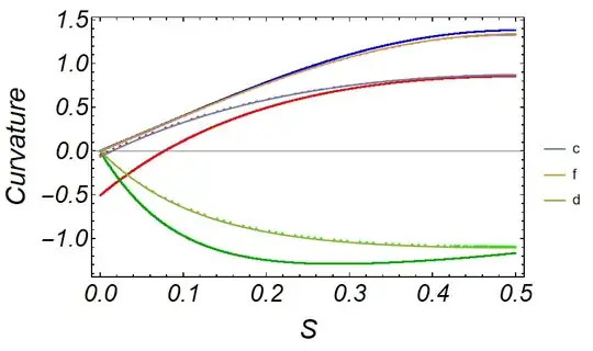
These data (doted lines) we can compare with sisRK4 results (solid lines) Figure 3

Note, the code above has not been tested for every run. If sol converges then it should be solution as above.

We can also solve this problem with parametric NDSolve. To avoid singularity at f->0, we use rule d/f=d'/f' at f->0, d->0. With this rule we solve equations at first step h = 10^-8. Therefore we have

    eq = With[{c = c[s], f = f[s], d = d[s]}, 
   D[{c, f, d}, s] - {(-2 d Sqrt[1 - f c^2])/f, 
     4 Sqrt[1 - 
        f c^2], -(2 c^2 (d - c0) + c (c0^2 - d^2) + (LK) c + dP + 
         4 d (1 - f c^2)/f)/Sqrt[1 - f c^2]}];
h = 10^-8; ic = { c[h] == p + h/4 (dP + c0^2 p + LK p - 2 c0 p^2), 
  f[h] == 4 h, d[h] == h/2 (-dP - c0^2 p - LK p + 2 c0 p^2)}; eq1 = 
 Join[Table[eq[[i]] == 0, {i, 3}], ic] /. {c0 -> -4, dP -> 1748/100};
sol1 = ParametricNDSolve[eq1, {c, f, d}, {s, h, 1/2}, {p, LK}];

cfun = c /. sol1; ffun = f /. sol1; dfun = d /. sol1; eqn = {cfun[p, LK][s] Sqrt[ffun[p, LK][s]] == 1, LK == 2 cfun[p, LK][s] (c0 - dfun[p, LK][s]) + dfun[p, LK][s]^2 - c0^2 - (dP/cfun[p, LK][s])} /. {c0 -> -4, dP -> 1748/100, s -> 1/2};

sol2 = FindRoot[eqn, {{p, -1/2}, {LK, -40}}, WorkingPrecision -> 30, MaxIterations -> 1000, Method -> {"Newton", "StepControl" -> "LineSearch"}] ({p -> -0.0684148292163831185884264856396, LK -> -39.9768774596520202382742346701})

Visualization

    Plot[Evaluate[
      Re[{cfun[p, LK][s], ffun[p, LK][s], dfun[p, LK][s]}] /. sol2], {s, 
      h, .5}, PlotLegends -> {"c", "f", "d"}, AxesLabel -> Automatic]

This solution (thin solid lines) consider with the Haar wavelets collocation method (dotted lines), but differ from sisRK4 Figure 4

Alex Trounev
  • 44,369
  • 3
  • 48
  • 106
  • thanks. Is the variable eqn defined above? the code seems to be crashing when I am running it. – Ali Hashmi Feb 27 '23 at 11:56
  • also Alex I was wondering whether the advanced NDSolve related functionality as listed here (https://reference.wolfram.com/language/tutorial/NDSolveStateData.html) can be used to compute LK from starting test values provided for c[0], c[0.5], d[0] before NDSolve computes anything else? – Ali Hashmi Feb 27 '23 at 12:34
  • Sorry, expression for eqn has been added. – Alex Trounev Feb 27 '23 at 13:25
  • Hi Alex, i think it is still missing. For the context i mean the variable eqn in eqs[y_] := -2 U1[y] + eqn ... is still not defined. thanks again – Ali Hashmi Feb 27 '23 at 13:30
  • @AliHashmi Thank you for testing, now it looks like working code. Please, see also update with ParametricNDSolve solution. – Alex Trounev Feb 27 '23 at 16:14
  • thanks Alex. actually with dP = 17.48 and c0=-4 the curves should look like this instead https://imgur.com/a/l8LZ6Sg. It is correct as it has been reported in literature as well and can be generated by the code i have posted in question. In your case why does c and d are essentially constants for all values of s? At the end of the procedure (not shown in the post) the curvature c is integrated to get the shape of the object. It certainly should not be a constant – Ali Hashmi Feb 27 '23 at 17:45
  • d is 0 at s=0 and f is 0 at s = 0 and we start from guess values x,y,z and improve our estimates of these values (see code in the question) until the boundary conditions are satisfied. sisRK4 is i guess the runge kutta scheme and the second part of the code (with Jacobian Matrix calculation) uses newton method to improve estimates of x,y,z. At least that is my thinking about the code in the question. – Ali Hashmi Feb 27 '23 at 18:00
  • @AliHashmi I think that we need additional restriction for this model. Could you give a link to the report with picture you show? – Alex Trounev Feb 28 '23 at 03:33
  • 1
    I have created a google drive folder and link for you. There are two articles that I placed inside. you can choose to read anyone you like (the code posted in the question belongs to one of the articles and is present in the supplementary folder associated with one of the articles and presents further detail on how the authors solve/implement the model) : https://drive.google.com/drive/folders/1UgTW3O0jSE5RTXOpkEeszw_nswuZMp_C?usp=sharing – Ali Hashmi Feb 28 '23 at 22:08
  • @AliHashmi Thank you for the model clarification. As I understand you used equations (41), (42), (43), (44) from American Journal of Physics 89, 465 (2021) and code they are proposed. – Alex Trounev Mar 02 '23 at 03:51
  • yes you are right. and equation 45 as well which are the boundary conditions to be satisfied. 44 is a constraint equation. and (41-43) are the main differential equations – Ali Hashmi Mar 06 '23 at 22:34
  • If so then you need to put f[0]==0 as in first equation (45). The difference between your solution with f[0][==10^-3 and my solution with f[0]==0 shown in Update 1 for my answer. – Alex Trounev Mar 07 '23 at 03:13
  • actually i am getting weird answers by running your scripts. I added ClearAll to remove any definitions and also tried to run your code in fresh kernel. I am getting strange answers. can you kindly check what is happening by running your code one by one in a fresh kernel – Ali Hashmi Mar 07 '23 at 13:30
  • @AliHashmi Sorry, some part of code has been removed occasionally. Please, test again. – Alex Trounev Mar 08 '23 at 05:38
  • the code runs now but the issue is in the last piece of code. try changing LK to -60 in your code and you will see that the root for LK deviates a lot. sol2 = FindRoot[eqn, {{p, -1/2}, {LK, -40}}, WorkingPrecision -> 30, MaxIterations -> 1000, Method -> {"Newton", "StepControl" -> "LineSearch"}] – Ali Hashmi Mar 08 '23 at 17:52
  • @AliHashmi Yes, you are right. Nevertheless, we can use two consider solutions from above to test your code. Also, please pay attention that your code not reproduces exact solution. – Alex Trounev Mar 09 '23 at 02:29
  • fair point. actually this is how my solution below compares with yours. https://imgur.com/oVyF33d – Ali Hashmi Mar 09 '23 at 09:55
  • @AliHashmi This is very good. Could you add this picture to your answer? Practically you have several codes for your future research. The only question is how to reproduce exact solution with your code? – Alex Trounev Mar 09 '23 at 12:57
  • thanks. i added the plots and accepted your answer, As for your question, it is also a fairly open question for me too. for now my purpose is to assume some dP and generate the different shapes – Ali Hashmi Mar 10 '23 at 15:16
  • 1
    Thank you very much. This is very useful discussion. – Alex Trounev Mar 11 '23 at 05:17
1

Below is how NDSolve can be modified to solve the model above. Although not the best or the most convenient implementation with the built-in function, The advanced features of NDSolve can give us control over changing the state of variable LK before computing anything else.

In crux, it is more or less the same code as the one I posted in the question with the only difference that I use NDSolve here to iterate the equations with CRK4 method than sisRK4 (in the question).

CRK4[{two_, half_, sixth_}]["Step"[rhs_, h_, t_, x_, xp_]] := 
  Module[{k4, k1, k2, k3},
   k1 = h xp;
   k2 = h rhs[t + half h, x + half k1];
   k3 = h rhs[t + half h, x + half k2];
   k4 = h rhs[t + h, x + k3];
   sixth (k1 + two (k2 + k3) + k4)
   ];

CRK4 /: NDSolve`InitializeMethod[CRK4, stepmode_, sd_, rhs_, state_, opts___] := Module[{prec}, prec = state@"WorkingPrecision"; CRK4[N[{2, 1/2, 1/6}, prec]] ] CRK4[___]["StepInput"] = {"F"["T", "X"], "H", "T", "X", "XP"}; CRK4[___]["StepOutput"] = "XI"; CRK4[___]["DifferenceOrder"] := 4 CRK4[___]["StepMode"] := Fixed

step = 0.0001; x = -0.8; y = 0.8; z = -0.6; c0 = -4.0; dP = 17.48;
[Beta] = True; hx = step; hy = step; hz = step;

While[[Beta], LK = 2 y (c0 - z) + (z)^2 - c0^2 - (dP/y); state = First@NDSolveProcessEquations[{c'[ s] - (-2 d[s] Sqrt[1 - f[s] c[s]^2])/f[s] == 0, f'[s] - 4 Sqrt[1 - f[s] c[s]^2] == 0, d'[ s] - (-(2 c[s]^2 (d[s] - c0) + c[s] (c0^2 - d[s]^2) + LK*c[s] + dP + 4 d[s] (1 - f[s] c[s]^2)/f[s]))/(Sqrt[ 1 - f[s] c[s]^2]) == 0, f[0] == 0.0001, c[0] == x, d[0] == 0.0}, {f, c, d}, {s, 0, 1/2}, Method -&gt; CRK4, StartingStepSize -&gt; 0.0005]; NDSolveIterate[state, 1/2]; sol = NDSolve`ProcessSolutions[state]; {fN, cN, dN} = {f[1/2], c[1/2], d[1/2]} /. sol;

f1 = Abs[y Sqrt[fN] - 1]; f2 = Abs[y - cN]; f3 = Abs[z - dN];

[Beta] = If[f1 < 0.001 && f2 < 0.001 && f3 < 0.001, False, True];

If[[Beta], {x2, y2, z2} = {x + hx, y + hy, z + hz};

LK = 2 y (c0 - z) + (z)^2 - c0^2 - (dP/y); state = First@NDSolveProcessEquations[{c'[ s] - (-2 d[s] Sqrt[1 - f[s] c[s]^2])/f[s] == 0, f'[s] - 4 Sqrt[1 - f[s] c[s]^2] == 0, d'[ s] - (-(2 c[s]^2 (d[s] - c0) + c[s] (c0^2 - d[s]^2) + LK*c[s] + dP + 4 d[s] (1 - f[s] c[s]^2)/f[s]))/(Sqrt[ 1 - f[s] c[s]^2]) == 0, f[0] == 0.0001, c[0] == x2, d[0] == 0.0}, {f, c, d}, {s, 0, 1/2}, Method -&gt; CRK4, StartingStepSize -&gt; 0.0005]; NDSolveIterate[state, 1/2]; sol = NDSolve`ProcessSolutions[state];

{fNx, cNx, dNx} = {f[1/2], c[1/2], d[1/2]} /. sol; f1x = Abs[y Sqrt[fNx] - 1]; f2x = Abs[y - cNx]; f3x = Abs[z - dNx];

LK = 2 y2 (c0 - z) + (z)^2 - c0^2 - (dP/y2); state = First@NDSolveProcessEquations[{c'[ s] - (-2 d[s] Sqrt[1 - f[s] c[s]^2])/f[s] == 0, f'[s] - 4 Sqrt[1 - f[s] c[s]^2] == 0, d'[ s] - (-(2 c[s]^2 (d[s] - c0) + c[s] (c0^2 - d[s]^2) + LK*c[s] + dP + 4 d[s] (1 - f[s] c[s]^2)/f[s]))/(Sqrt[ 1 - f[s] c[s]^2]) == 0, f[0] == 0.0001, c[0] == x, d[0] == 0.0}, {f, c, d}, {s, 0, 1/2}, Method -&gt; CRK4, StartingStepSize -&gt; 0.0005]; NDSolveIterate[state, 1/2]; sol = NDSolve`ProcessSolutions[state];

{fNy, cNy, dNy} = {f[1/2], c[1/2], d[1/2]} /. sol; f1y = Abs[y2 Sqrt[fNy] - 1]; f2y = Abs[y2 - cNy]; f3y = Abs[z - dNy];

LK = 2 y (c0 - z2) + (z2)^2 - c0^2 - (dP/y); state = First@NDSolveProcessEquations[{c'[ s] - (-2 d[s] Sqrt[1 - f[s] c[s]^2])/f[s] == 0, f'[s] - 4 Sqrt[1 - f[s] c[s]^2] == 0, d'[ s] - (-(2 c[s]^2 (d[s] - c0) + c[s] (c0^2 - d[s]^2) + LK*c[s] + dP + 4 d[s] (1 - f[s] c[s]^2)/f[s]))/(Sqrt[ 1 - f[s] c[s]^2]) == 0, f[0] == 0.0001, c[0] == x, d[0] == 0.0}, {f, c, d}, {s, 0, 1/2}, Method -&gt; CRK4, StartingStepSize -&gt; 0.0005]; NDSolveIterate[state, 1/2]; sol = NDSolve`ProcessSolutions[state];

{fNz, cNz, dNz} = {f[1/2], c[1/2], d[1/2]} /. sol; f1z = Abs[y Sqrt[fNz] - 1]; f2z = Abs[y - cNz]; f3z = Abs[z2 - dNz];

Jf = ( { {(f1x - f1)/hx, (f1y - f1)/hy, (f1z - f1)/hz}, {(f2x - f2)/hx, (f2y - f2)/hy, (f2z - f2)/hz}, {(f3x - f3)/hx, (f3y - f3)/hy, (f3z - f3)/hz} } );

{x, y, z} = {x, y, z} - Inverse[Jf] . {f1, f2, f3}; ]; ]; Print@{LK, {x, y, z}};

({-39.9958,{-0.0887335,0.864286,-1.10808}})

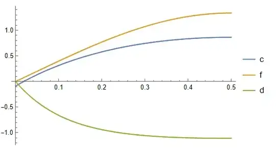
ListLinePlot[Evaluate[{c, f, d} /. sol], PlotStyle -> {"c", "f", "d"}]

enter image description here

also this compares fairly well with the solution posted by @Alex Trounev

enter image description here

Ali Hashmi
  • 8,950
  • 4
  • 22
  • 42
  • Did you try to make a research with this code, for example, how solution converges with step decreasing? – Alex Trounev Mar 02 '23 at 03:54
  • @AlexTrounev no actually I did not change the step. I merely compared the answer here with the one I got from the code in the question. Essentially used NDSolve as the iterator here. Does it change in your opinion? – Ali Hashmi Mar 06 '23 at 22:37
  • Actually your code is very good (+1) compare to published in the paper. My question is only about boundary condition f[0]==10^-3 you used, while in the paper they used f[0]==0. – Alex Trounev Mar 07 '23 at 03:45
  • But this method is very sensitive to the step size decreasing. For example, for StartingStepSize -> 5 10^-5 we have {-39.7464,{-0.443645,0.854412,-1.21378}}, while for StartingStepSize -> 5 10^-4 as above we have {-39.8661,{-0.517524,0.852474,-1.19337}}. Therefore solution is not converged. – Alex Trounev Mar 07 '23 at 04:07
  • Also for StartingStepSize -> 2 10^-5 we have {-39.9449,{-0.380249,0.853735,-1.16829}}, and c[0] /. sol is about -0.380249 compare to -0.506871 at StartingStepSize -> 5 10^-4 . Generally speaking we need to update this code so that the numerical solution converges with step size decreasing. – Alex Trounev Mar 07 '23 at 04:34
  • @AlexTrounev I have updated this code and now I think it agrees fairly well with yours. I modified the step variable to a lower value like 0.0001 as it was being used to computes the derivatives in the Jacobian during the Newton Method (via hx, hy and hz which were all set to the value of the step variable). Reducing it gives a fairly nice agreement with your answer. Of course I have also lowered f[0] to an even lower value but did not get a 100 percent agreement. I cannot use f[0]=0 in this formulation as we get an indeterminate form. – Ali Hashmi Mar 07 '23 at 11:44
  • 1
    Thank you very much. Now solution converges with step size decreasing to that we computed with the Euler wavelet collocation method. – Alex Trounev Mar 07 '23 at 12:52