Stefan problem with mixed bc

Question

I am trying to solve through Mathematica the classical Stefan problem $$ \left\{ \begin{array}{lll} \dot{v}(x,t)=v_{xx}(x,t) & x\in(0,s(t))\\ \dot{s}(t)=-v_x(s(t),t) & x = s(t)\\ v(0,t) = 0 & x = 0\\ v(x,0) = v_0(x) & \\ \end{array} \right. $$ with the novelty that the boundary condition on the moving front is not the usual $v(s(t),t)=0$, but rather $$ \displaystyle\color{red}{v_x(s(t),t) - \frac{1}{s(t)} v(s(t),t) = F(t)} $$ with $F(t)$ some given function. I have tried to understand how the great answer of @ybeltukov could be modified, even (say) in the simple case of $$ F(t)=t, \qquad v_0(x)=x $$ But I have been scratching my head uselessly for days ... I hope somebody could give me a grind on this!

Thanks so much!

There're many other related posts in this site, e.g. https://mathematica.stackexchange.com/q/211080/1871 (Don't miss the links in comment), have you read them? — xzczd, Mar 23 '23 at 03:07
Hi @xzczd, I think I've spent the whole week to read the various posts and suggested method of implementation of Stefan problem; nobody considers general types of bc on the moving front. Which is crucial for my research ... :/ — Josè, Mar 23 '23 at 09:32
I don't think there's anything special in your b.c., it's merely a Robin b.c. involving $s(t)$ term. Please think carefully about change of variable, and play with DChange/DSolveChangeVariables. — xzczd, Mar 23 '23 at 09:43
Another related post: https://mathematica.stackexchange.com/a/269866/1871 — xzczd, Mar 23 '23 at 09:52
It is not clear what initial condition $v_0(x)=x$ means in this case? If $0\le x\le s(t)$ and $s(0)=0$ then $v_0(x)=0$. Should we suppose that $s(0)>0$? — Alex Trounev, Mar 23 '23 at 13:01
@AlexTrounev, in my specific case I will assume $v_0(x)=0$, but I was just willing to think of the possibility that this is not the case, as far as I am aware in PDEs the initial condition ought not to be $v_0(x)=0$; also note this looks like Stefan problem but it isn't so. — Josè, Mar 23 '23 at 14:32
and thanks so much for sharing the specific location of pertinent comments, I had not understood that these contain elements to adapt @ybeltukov ' solution to embed Robin's conditions. I will give it a try and get back .... but thanks for now! — Josè, Mar 23 '23 at 14:34

Alex Trounev · Answer 1 · 2023-03-26T11:24:21.573

This problem can be solved with using the Euler wavelets collocation method as follows. We introduce same normalized variable as here in the form $x\rightarrow \frac {x}{s(t)}$. First, we test code utilizing numerical solution from @ybeltukov answer

OEm[m_, x_] := 
 Sqrt[2 m + 
    1] Sum[(-1)^(m - k) x^k Binomial[m, k] Binomial[m + k, k], {k, 0, 
    m}]; UE[m_, t_] := OEm[m, t];
psi[k_, n_, m_, t_] := 
 Piecewise[{{2^((k - 1)/2) UE[m, 2^(k - 1) t - n + 1], (n - 1)/
      2^(k - 1) <= t < n/2^(k - 1)}, {0, True}}]; 
PsiE[k_, M_, t_] := 
 Flatten[Table[psi[k, n, m, t], {n, 1, 2^(k - 1)}, {m, 0, M - 1}]]
k0 = 3; M0 = 4;
With[{k = k0, M = M0}, 
  nn = Length[Flatten[Table[1, {n, 1, 2^(k - 1)}, {m, 0, M - 1}]]]];
dx = 1/(nn); xl = Table[l*dx, {l, 0, nn}]; xcol = 
 Table[(xl[[l - 1]] + xl[[l]])/2, {l, 2, nn + 1}];
Psijk = With[{k = k0, M = M0}, PsiE[k, M, t1]]; Int1 = 
 With[{k = k0, M = M0}, Integrate[PsiE[k, M, t1], t1]];
Int2 = Integrate[Int1, t1];
Psi[y_] := Psijk /. t1 -> y;
int1[y_] := Int1 /. t1 -> y;
int2[y_] := Int2 /. t1 -> y;
wA = Table[wa[i][t], {i, nn}]; wB = Table[wb[i][t], {i, 2}];
v2[x_] := wA . Psi[x]; v1[x_] := wA . int1[x] + wB[[1]];
v0[x_] := wA . int2[x] + wB[[1]] x + wB[[2]];
equ = {D[v0[x], t] + (x v1[1] v1[x])/s[t]^2 == v2[x]/
   s[t]^2}; eqnS = {s'[t] == -v1[1]/s[t]};
eqx = Table[equ, {x, xcol}];
eqs = Join[Flatten[eqx], eqnS];
bc = Join[{v1[0] + s[t] == 0}, {v0[1] == 0}]; icx = {v0[x] == 0 /. 
   t -> 0}; ic = Table[icx, {x, xcol}] // Flatten;
varAll = Join[wA, wB, {s[t]}];
icn = Join[ic, bc /. t -> 0, {s[0] == 10^-3}]; eqnN = 
 Join[eqs, D[bc, t]]; var1 = D[varAll, t];
{vec, mat} = CoefficientArrays[eqnN, var1];
f = Inverse[mat // N] . (-vec);
vr0 = varAll /. t -> 0; {w0, mat0} = CoefficientArrays[icn, vr0];
s0 = Inverse[mat0 // N] . (-w0); rul0 = 
 Table[vr0[[i]] -> s0[[i]], {i, Length[vr0]}];
f0 = f /. t -> 0 /. rul0; m = Length[f];
sol = NDSolve[{Table[var1[[i]] == f[[i]], {i, Length[var1]}], 
    Table[vr0[[i]] == s0[[i]], {i, Length[vr0]}]}, varAll, {t, 0, 1}];

Visualization and comparison with @ybeltukov solution (dashed lines)

lst = Table[{{t, x}, v0[x] /. sol[[1]]}, {t, 0, 1, .1}, {x, 0, 
   1, .1}]; u = Interpolation[Flatten[lst, 1]]; S = 
 Interpolation[Table[{t, s[t] /. sol[[1]]}, {t, 0, 1, .01}]];
{Show[{DensityPlot[
   u[t, x/S[t]] UnitStep[S[t] - x], {t, 0, 1}, {x, 0, 1}, 
   FrameLabel -> {"t", "x"}, ColorFunction -> "Rainbow"], 
  Plot[s[t] /. sol[[1]], {t, 0, 1}, PlotStyle -> {Red, Dashed}]}],Plot[{u[t, 0], u[1, t/S[1]] UnitStep[S[1] - t], S[t]}, {t, 0, 1}, 
 PlotLegends -> Automatic, Frame -> True, 
 PlotStyle -> {Red, Blue, Black}]}

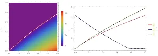
Note, that two numerical solution are in a good agreement, therefore we can try to solve problem proposed by Josè. In this case we consider solution with initial data $v(x,0)=vini(x)=x, s(0)=3$, we have

s0 = 3; F[t_] := t; vini[x_] := x; tmax = 1.;
OEm[m_, x_] := 
 Sqrt[2 m + 
    1] Sum[(-1)^(m - k) x^k Binomial[m, k] Binomial[m + k, k], {k, 0, 
    m}]; UE[m_, t_] := OEm[m, t];
psi[k_, n_, m_, t_] := 
  Piecewise[{{2^((k - 1)/2) UE[m, 2^(k - 1) t - n + 1], (n - 1)/
       2^(k - 1) <= t < n/2^(k - 1)}, {0, True}}];
PsiE[k_, M_, t_] := 
 Flatten[Table[psi[k, n, m, t], {n, 1, 2^(k - 1)}, {m, 0, M - 1}]]
k0 = 3; M0 = 4;
With[{k = k0, M = M0}, 
  nn = Length[Flatten[Table[1, {n, 1, 2^(k - 1)}, {m, 0, M - 1}]]]];
dx = 1/(nn); xl = Table[l*dx, {l, 0, nn}]; xcol = 
 Table[(xl[[l - 1]] + xl[[l]])/2, {l, 2, nn + 1}];
Psijk = With[{k = k0, M = M0}, PsiE[k, M, t1]]; Int1 = 
 With[{k = k0, M = M0}, Integrate[PsiE[k, M, t1], t1]];
Int2 = Integrate[Int1, t1];
Psi[y_] := Psijk /. t1 -> y;
int1[y_] := Int1 /. t1 -> y;
int2[y_] := Int2 /. t1 -> y;
wA = Table[wa[i][t], {i, nn}]; wB = Table[wb[i][t], {i, 2}];
v2[x_] := wA . Psi[x]; v1[x_] := wA . int1[x] + wB[[1]];
v0[x_] := wA . int2[x] + wB[[1]] x + wB[[2]];
equ = {D[v0[x], t] + (x v1[1] v1[x])/s[t]^2 == 
   v2[x]/s[t]^2}; eqnS = {s'[t] == -v1[1]/s[t]};
eqx = Table[equ, {x, xcol}];
eqs = Join[Flatten[eqx], eqnS];
bc = Join[{v0[0] == 0}, {v1[1] - v0[1] == s[t] F[t]}]; icx = {v0[x] ==
     vini[x] s0 /. t -> 0}; ic = Table[icx, {x, xcol}] // Flatten;
varAll = Join[wA, wB, {s[t]}];
icn = Join[ic, bc /. t -> 0, {s[0] == s0}]; eqnN = 
 Join[eqs, D[bc, t]]; var1 = D[varAll, t];
f = var1 /. Solve[eqnN, var1][[1]];
vr0 = varAll /. t -> 0; s00 = vr0 /. Solve[icn, vr0][[1]];
sol = NDSolve[{Table[var1[[i]] == f[[i]], {i, Length[var1]}], 
    Table[vr0[[i]] == s00[[i]], {i, Length[vr0]}]}, 
   varAll, {t, 0, tmax}];

Visualization

S = Interpolation[
  Table[{t, s[t] /. sol[[1]]}, {t, 0, tmax, .01}]]; lst = 
 Table[{{t, x}, v0[x] /. sol[[1]]}, {t, 0, tmax, .05}, {x, 0, 
   1, .05}];
Show[{DensityPlot[
   u[t, x/S[t]] UnitStep[S[t] - x], {t, 0, tmax}, {x, 0, S[tmax]}, 
   FrameLabel -> {"t", "x"}, ColorFunction -> "Rainbow", 
   PlotRange -> All, PlotLegends -> Automatic], 
  Plot[S[t], {t, 0, tmax}, PlotStyle -> {Red, Dashed}, 
   PlotRange -> All]}]

Update 1. Second method to solve this problem is FDM, same as @ybeltukov, but much clear

ns = 101; h = 1/(ns - 1);
x[t_] = Table[Symbol["x" <> ToString[i]][t], {i, 1, ns}];
xgrid = Table[k h, {k, 0, ns - 1}]; M2 = 
 NDSolve`FiniteDifferenceDerivative[Derivative[2], xgrid, 
   DifferenceOrder -> 2]@"DifferentiationMatrix"; M1 = 
 NDSolve`FiniteDifferenceDerivative[Derivative[1], xgrid, 
   DifferenceOrder -> 2]@"DifferentiationMatrix";
eqnS = {s'[t] == -(M1 . x[t])[[ns]]/s[t]}; eq = 
 Table[(D[x[t], t])[[i]] + 
    xgrid[[i]] (M1 . x[t])[[ns]] (M1 . x[t])[[i]]/
      s[t]^2 == (M2 . x[t])[[i]]/s[t]^2, {i, 2, ns - 1}];
bc = {(M1 . x[t])[[1]] == -s[t], x[t][[ns]] == 0};
ini = Join[{s[0] == .001}, Table[x[0][[i]] == 0, {i, 2, ns - 1}]];
sol = NDSolve[{Join[eqnS, eq, D[bc, t]], Join[ini, bc /. t -> 0]}, 
   Join[{s[t]}, x[t]], {t, 0, 1}];

Visualization and comparison with previous solution (dashed lines)

u = Interpolation[
  Flatten[Table[{{t, xgrid[[i]]}, x[t][[i]] /. sol[[1]]}, {t, 0, 
     1, .1}, {i, ns}], 1]];
S = Interpolation[Table[{t, s[t] /. sol[[1]]}, {t, 0, 1, .001}]];
{Show[{DensityPlot[
   u[t, x/S[t]] UnitStep[S[t] - x], {t, 0, 1}, {x, 0, 1}, 
   FrameLabel -> {"t", "x"}, ColorFunction -> "Rainbow"], 
  Plot[S[t], {t, 0, 1}, PlotStyle -> {Red, Dashed}]}],Plot[{u[t, 0], u[1, t/S[1]] UnitStep[S[1] - t], S[t]}, {t, 0, 1},
Frame -> True, PlotStyle -> {Red, Green, Blue}, 
 PlotLegends -> Automatic]}

Finally we can solve problem proposed by Josè with initial data $v(x,0)=v_0(x)=x,s(0)=3$, and for $F(t)=t$, we have

F[t_] := t; v0[x_] := x;
ns = 101; h = 1/(ns - 1);
x[t_] = Table[Symbol["x" <> ToString[i]][t], {i, 1, ns}];
xgrid = Table[k h, {k, 0, ns - 1}]; M2 = 
 NDSolveFiniteDifferenceDerivative[Derivative[2], xgrid, DifferenceOrder -&gt; 2]@&quot;DifferentiationMatrix&quot;; M1 = NDSolveFiniteDifferenceDerivative[Derivative[1], xgrid, 
   DifferenceOrder -> 2]@"DifferentiationMatrix";
eqnS = {s'[t] == -(M1 . x[t])[[ns]]/s[t]}; eq = 
 Table[(D[x[t], t])[[i]] + 
    xgrid[[i]] (M1 . x[t])[[ns]] (M1 . x[t])[[i]]/
      s[t]^2 == (M2 . x[t])[[i]]/s[t]^2, {i, 2, ns - 1}];
bc = {(M1 . x[t])[[ns]] - x[t][[ns]] == s[t] F[t], x[t][[1]] == 0};
ini = Join[{s[0] == 3}, 
   Table[x[0][[i]] == 3 v0[xgrid[[i]]], {i, 2, ns - 1}]];
sol = NDSolve[{Join[eqnS, eq, D[bc, t]], Join[ini, bc /. t -> 0]}, 
   Join[{s[t]}, x[t]], {t, 0, 1}];

Visualization and comparison with wavelets solution (dashed lines)

Show[{DensityPlot[
   u[t, x/S[t]] UnitStep[S[t] - x], {t, 0, 1}, {x, 0, 3}, 
   FrameLabel -> {"t", "x"}, ColorFunction -> "Rainbow"], 
  Plot[S[t], {t, 0, 1}, PlotStyle -> {Red, Dashed}]}];
Plot[{u[1, t/S[1]] UnitStep[S[t] - t], S[t]}, {t, 0, 1}, 
 PlotStyle -> Dashed, PlotLegends -> Automatic];
u = Interpolation[
  Flatten[Table[{{t, xgrid[[i]]}, x[t][[i]] /. sol[[1]]}, {t, 0, 
     1, .1}, {i, ns}], 1]];

S = Interpolation[Table[{t, s[t] /. sol[[1]]}, {t, 0, 1, .001}]];

{Show[{DensityPlot[
   u[t, x/S[t]] UnitStep[S[t] - x], {t, 0, tmax}, {x, 0, s0}, 
   FrameLabel -> {"t", "x"}, ColorFunction -> "Rainbow", 
   PlotRange -> All, PlotLegends -> Automatic], 
  Plot[S[t], {t, 0, tmax}, PlotStyle -> {Red, Dashed}, 
   PlotRange -> All]}],Plot[{u[1, t/S[1]] UnitStep[S[t] - t], S[t]}, {t, 0, 1}, 
 PlotStyle -> {Red, Blue}, PlotLegends -> Automatic]}

But this is just amazing! you can not even imagine how grateful am I …. I would have NEVER arrived here! I will play with it and will give feedback on how it goes :) thanks heathfully! — Josè, Mar 24 '23 at 15:51
Ok so. The 1st part where you redo the solution of the Stefan problem is ok. 2nd part where you solve my problem doesn't run on my machine (Mathematica 12). Specifically the (first) problematic line is: f = Inverse[mat // N].(-vec); Delivering several: General::munfl: 1.493*10^-237 (-7.40643*10^-238) is too small to represent as a normalized machine number; precision may be lost. altogether with: Inverse::sing: Matrix {<<1>>} is singular. Any clue? Thanks so much ... — Josè, Mar 25 '23 at 12:26
Ah, I see that last part has no definition for S, u (done). Also, please run second part on the fresh kernel. — Alex Trounev, Mar 25 '23 at 13:28
thanks so much for your patience. The problem is before that line, my first errors are immediately after f = Inverse[mat // N].(-vec);delivering the error messages of previous message (notably Inverse::sing: Matrix {<<1>>} is singular.) ... any clue? :/ — Josè, Mar 25 '23 at 14:34
@Josè Fortunately I have v12 on my old computer. I have tested code and found out error due to matrix inversion. Solution computed with new code using Solve shown above. — Alex Trounev, Mar 25 '23 at 16:55
Hi Alex Tournev, I have pretty much followed everything of your last implementation (fantastic!), apparently in your code for my problem the definition of u was still missing, I've added it as u = Interpolation[Flatten[lst, 1]];. Now the code runs but the graphics isn't like yours as the plot of the u(t,x) function stops half way, also I get some errors after my added line for u, Flatten::normal: Nonatomic expression expected at position 1 in Flatten[lst,1]. and Interpolation::innd: First argument in Flatten[lst,1] does not contain a list of data and coordinates., any suggestion? Thanks! — Josè, Mar 26 '23 at 11:10
PS it may actually have to do with my v12 Mathematica version, as I've plotted with x in (0,3) instead of x in (x,s(tmax)) and it now plots great! :) Thanks so much Alex! PS: if you like please add the u = Interpolation[Flatten[lst, 1]]; code line as it's missing in the final solution of my problem, so maybe others in future will have no problem! :) thanks so much again! — Josè, Mar 26 '23 at 11:18
thanks for this MASSIVE help, I've checked also the FDM method, both work now, my personal favorite at this point is the previous pone you had posted, which was very clean and I know where/how to play to modify the equation! Have a lovely Sunday and thanks immensely!!! — Josè, Mar 26 '23 at 11:59
Thanks to your answer, I noticed my "moving grid method" is wrong 囧. Just spent 2 hours to revise all the related posts. (Of course +1. ) — xzczd, Apr 24 '23 at 13:10

xzczd · Answer 2 · 2023-04-24T15:24:30.520

Let me add my FDM solution. The spirit of this solution is the same as that of Alex's FDM solution, except that the process is automated with pdetoode and DChange. Since there's nothing new in the following code compared to the previous moving boundary problems in this site, I won't explain much. (Anyway, if you still feel it difficult to follow, feel free to ask in the comment, but please be specific. )

I've chosen the same initial data as in Alex's answer so we can easily verify the result.

s0 = 3;
F = t; v0 = x;
With[{v = v[x, t], 
   s = s[t]}, {eq, ic, 
    bc} = {{D[v, t] == D[v, x, x], 
     D[s, t] == -D[v, x] /. x -> s}, {v == v0, s == s0} /. t -> 0, {v == 0 /. x -> 0,
      D[v, x] - 1/s v == F /. x -> s}}];
(* Definition of DChange isn't included in this post,
   please find it in the link above. *)       
{neweq, newicmid, newbc} = DChange[{eq, ic, bc}, x/s[t] == ξ, x, ξ, v[x, t]]    
newic = {newicmid[[1]] /. t -> 0 /. s[0] -> s0, newicmid[[2]]};
With[{ic = newic, eq = neweq, bc = newbc},
 domain = {0, 1}; points = 25; grid = Array[# &, points, domain]; difforder = 2;
  (* Definition of pdetoode isn't included in this post,
     please find it in the link above. *)
  ptoofunc = pdetoode[v[ξ, t], t, grid, difforder];
  del = #[[2 ;; -2]] &;
ode = {del@ptoofunc@eq[[1]], ptoofunc@eq[[2]]};
  odebc = ptoofunc@bc;
  odeic = {ic[[1]] // ptoofunc // del, ic[[2]]} /. t -> 0;
  tend = 1;
  {ssol, vsollst} = 
   NDSolveValue[{ode, odeic, odebc}, {s, v /@ grid}, {t, 0, tend}]; // AbsoluteTiming]
vscaledsol = rebuild[vsollst, grid, 2];
vsol = {x, t} |-> vscaledsol[x/ssol[t], t];
reg = DiscretizeRegion@ImplicitRegion[x <= ssol[t], {{t, 0, 1}, {x, 0, 3}}];
DensityPlot[vsol[x, t], {t, x} ∈ reg]

Manipulate[
 Plot[vsol[x, t], {x, 0, ssol[t]}, PlotRange -> {{0, s0}, {-1, 5}}], {t, 0, 1}]

Thank you. It is nice application of your perfect code pdetoode (+1). — Alex Trounev, Apr 24 '23 at 14:22

Stefan problem with mixed bc

2 Answers2