13

I want to solve the one-dimensional one-phase Stefan problem, but I don't know how to make Mathematica understand the conditions.

If you are not familiar with what I'm asking please refer to this wikipedia article: http://en.wikipedia.org/wiki/Stefan_problem#Mathematical_formulation

This is what I have so far. Clearly, it doesn't work.

NDSolve[
 {D[u[x, t], t] == D[u[x, t], {x, 2}],
  (-D[u[x, t], x] /. x -> 0) == 1,
  u[s[t], t] == 0,
  D[s[t]] == (-D[u[x, t], x] /. x -> s[t]),
  u[x, 0] == 0,
  s[0] == 0
  },
{u, s}, {x, 0, s[t]}, {t, 0, 10}]

I hope there is someone out there with a magical code

I'm using Mathematica 10.

Thanks!

user21
  • 39,710
  • 8
  • 110
  • 167
Ivan
  • 2,207
  • 15
  • 25
  • 2
    http://www.sciencedirect.com/science/article/pii/S0307904X05001150 – Dr. belisarius Sep 01 '14 at 06:42
  • 1
    D[s[t]] should be s'[t]. (Of course this won't solve your problem… ) – xzczd Sep 01 '14 at 08:51
  • I just cannot understand the the basic thing. There is a well-known Stephan problem. It is solved a century ago. The solution is known in the analytical form. One can look here: Tychonoff, A. N. & Samarski, A. A. in Differentialgleichungen der mathematischen Physik 248-252 (Deutscher Verlag der Wissenschaften, Berlin, 1959). It also exists in English, then the names are A. N. Tikhonov and A. A. Samarskii, but then I cannot give the exact pages. – Alexei Boulbitch Sep 02 '14 at 07:33
  • 1
    Continuation: Now in the statement of Ivan Vladimir Gonzalez Bust I could not identify anything new with respect to the classical 1D Stephan problem. Did I miss something important. If not, why the author does not want to take the known solution? – Alexei Boulbitch Sep 02 '14 at 07:35
  • @AlexeiBoulbitch I suppose that it's just a simple example for a equation with the moving boundary. – ybeltukov Sep 02 '14 at 16:40
  • I was trying to figure out if Mathematica could handle this type of equations, with the simplest of the examples. – Ivan Sep 04 '14 at 18:24

2 Answers2

16

One can do it semi-automatically. Let us introduce a normalized variable $$ \xi = \frac{x}{s(t)}, \quad \xi \in [0,1] $$ and make a simple finite difference method over $\xi$.

The differential equation in new variables is

ClearAll[u, s, x, t, ξ]
D[u[x/s[t], t], t] == D[u[x/s[t], t], x, x] /. x -> ξ s[t]

enter image description here

If we divide the interval $[0,1]$ by $n$ subintervals we come to the following finite difference scheme

n = 100;
δξ = 1./n;

ClearAll[dv, t];
dv[v_List] := With[{s = First@v, u = Rest@v},
   With[{ds = u[[-1]]/(s δξ),
     ξ = N@Range[n - 1]/n,
     d1 = ListCorrelate[{-0.5, 0, 0.5}/δξ, #] &,
     d2 = ListCorrelate[{1, -2, 1}/δξ^2, #] &},
    Prepend[d2[#]/s^2 + ξ ds d1[#]/s &@Join[{u[[1]] + s δξ}, u, {0.}], ds]
    ]];
s0 = 0.001;
v0 = Prepend[ConstantArray[0., n - 1], s0];
sol = NDSolve[{v'[t] == dv[v[t]], v[0] == v0}, v, {t, 0, 1}][[1, 1, 2]];

Here v contains s (the first element) and u (the rest list).

It remains only to decompose the interpolation function sol and return to the initial variable x

Needs@"DifferentialEquations`InterpolatingFunctionAnatomy`";
values = InterpolatingFunctionValuesOnGrid@sol;
valu = Transpose@Join[{#[[2]] + δξ #[[1]]}, Rest@#, {0 #[[1]]}] &@
   Transpose@InterpolatingFunctionValuesOnGrid@sol;
vals = InterpolatingFunctionValuesOnGrid[sol][[All, 1]];
t = Flatten@InterpolatingFunctionGrid@sol;
ξ = Range[0., n]/n;
s = ListInterpolation[vals, t];
uξ = ListInterpolation[valu, {t, ξ}];
u = If[#2 < s[#], uξ[#, #2/s[#]], 0.] &;

Visualization of the result

Show[{DensityPlot[u[t, x], {t, 0, 1}, {x, 0, 1}, FrameLabel -> {"t", "x"}], 
   Plot[s[t], {t, 0, 1}, PlotStyle -> {Red, Dashed}]}]

enter image description here

ybeltukov
  • 43,673
  • 5
  • 108
  • 212
  • Er… why does u[ξ, t] still obey the heat equation? – xzczd Sep 02 '14 at 01:36
  • @xzczd u[ξ,t] obeys another equation (the first formula in the post). I have checked that resulting u[x,t] obeys the initial heat equation. – ybeltukov Sep 02 '14 at 02:00
  • Oh, I made a mistake… In fact, I mean why does u[x/s[t], t] obey the heat equation i.e. D[u[x/s[t], t], t] == D[u[x/s[t], t], x, x] is true? – xzczd Sep 02 '14 at 02:20
  • @xzczd, yes, it is true! I just expanded the derivatives in this equation. – ybeltukov Sep 02 '14 at 02:36
  • 1
    Ah, I understand! Here's a (relatively) detailed derivation: ReleaseHold[Hold[D[U[x, t], x, x] == D[U[x, t], t]] /. U[x, t] -> u[ξ[x, t], t] /. ξ[x, t] -> x/s[t]] /. x -> ξ s[t] (Alternative: D[U[x, t], x, x] == D[U[x, t], t] /. U -> ({x, t} \[Function] u[ξ[x, t], t]) /. ξ -> ({x, t} \[Function] x/s[t]) /. x -> ξ s[t] ) – xzczd Sep 02 '14 at 03:24
  • Thank you for your answer. So I guess Mathematica's NDSolve can't handle this type of problems automatically (?) – Ivan Sep 03 '14 at 04:40
  • @ybeltukov Thanks for your answer to this. I am amending your solution to fit another moving boundary problem. My PDE is slightly different $ h_t = \partial_x (h^3 h_x )$, but I think I know how to make this amend. However, the issue I have is with the moving boundary condition. Mine is slightly different: $\dot{s} = -u^2 u _x$. In your code I believe you incorporate OPs $\dot{s} = -u_x$ condition in this ds = u[[-1]]/(s δξ) statement, however I cannot see how to amend this statement for my slightly different moving BC. Could you make a suggestion? – mch56 May 16 '16 at 20:54
  • @ybeltukov Also, if I may ask, where in your solution do you satisfy the $-u_x (0,t) = 1$ condition ? – mch56 May 17 '16 at 15:08
  • @ojlm I assume $u=0$ for $x>s(t)$ so u[[-1]] represents the derivative $u_x$ at the boundary. May be you can write something like u[[-1]]^2(u[[-1]]-u[[-2]]). – ybeltukov May 18 '16 at 19:49
  • @ybeltukov I understand so u[[-1]] represents the derivative, because of the forward difference formula. So I can see how you have satisfied $s_t = -u_x$ with the line ds = u[[-1]]/(s δξ). How did you satisfy $-u_x(0,t) = 1$? I can't seem to see that line anywhere in the code? – mch56 May 19 '16 at 16:26
  • @ojlm The main line is Join[{u[[1]] + s δξ}, u, {0.}]. I add two points at both ends of the list u and then I take the derivatives. The term s δξ corresponds to $u_x=-1$. In the general case $u_x=-f(t)$ you can write f[t] s δξ. – ybeltukov May 20 '16 at 18:35
  • @ybeltukov Thanks for the response. I have successfully amended your code for a simple problem. However, I have one further question. I am now trying to extend the code to have two moving BCs. Discretised they are ds1 and ds2 say. I make similar amends as before, however when I amend this line Prepend[d2[#]/s^2 + ξ ds d1[#]/s &@Join[{u[[1]] + s δξ}, u, {0.}], ds] I amend it to Flatten@Prepend[eqns &@Join[{1}, u, {0.}], {ds1,ds2}] to incorporate the two moving BCs. I get a computed – mch56 May 23 '16 at 13:50
  • @ybeltukov derivatives do not have dimensionality consistent with the initial conditions. I think I'm not understanding why, in your original code, you need to Prepend the derivatives with the dsand thus not understanding how to extend it for two moving BCs. – mch56 May 23 '16 at 13:51
14

On the original question of how to solve classic Stefan-type problems using NDSolve with its high-level syntax (referred to in the posts as 'automatically'). This can be done. Essentially, first reformulate the problem as an optimal stopping problem: see van Moerbeke, Rocky Mountain J. Math. 4(3), 539-578, 1974. This leads to problems very similar to early exercise problems in Mathematical Finance. To solve these types of problems automatically with NDSolve, you can employ the WhenEvent methodology. Details are found in my recent book, "Option Valuation under Stochastic Volatility II", including a classic Stefan problem example. In Chapter 9, I treat a Stefan-type problem that is similar to, but not identical to the original question, namely: $$ \begin{align} w_{\tau} &= \frac{1}{2} w_{xx}, \quad x \in (s(\tau),\infty), \\ w(x,0) &= k \, 1_{\{x \ge 0 \}}, \quad (k > 0), \\ w(s(\tau),\tau) &= 0, \\ w_x(s(\tau),\tau) &= -2 \dot{s}(\tau). \end{align} $$ 
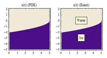
Here $w(x,\tau)$ is the water temperature for a water-ice phase transition and $s(\tau) \le 0$ is the moving boundary, which starts at $s(0)=0$.

The associated optimal stopping problem, using van Moerbeke, is $$ \begin{align} u_{\tau} &= \frac{1}{2} u_{xx}, \quad x \in (s(\tau),\infty), \\ u(x,0) &= (k+1) x^2 \, 1_{\{x > 0 \}}, \\ u(s(\tau),\tau) &= \tau, \\ u_x(s(\tau),\tau) &= 0. \end{align} $$

My main solver routine for the second problem is:

solverStefan[T_,k_,nexoppsperyear_,initsoln_,xmin_,xmax_,npts_]:=
Module[{xgrid,Soln,h,dt,hsoln,ecnt=0},
xgrid = xmin+(xmax-xmin)N[Table[i/npts,{i,0,npts}]]; 
dt = N[1/nexoppsperyear];
Soln =
 h/.NDSolve[{D[h[x,t],t] == 0.5 D[h[x,t],{x,2}],
 h[x,0] == initsoln[x],h[xmin,t] == t, h[xmax,t] == (k+1)(xmax^2+t),
 WhenEvent[Mod[t,dt] == 0, ecnt++;
 hsoln[x1_] := Max[h[x1,t], t];
 h[x,t]->Outer[hsoln[#1]&,xgrid]]},{h},{x,xmin,xmax},{t,0,T}, (* MUST USE {t,0,T} *)
  MaxSteps->1000000, MaxStepFraction->Min[dt/(10 T),1/npts],
  Method->{"MethodOfLines",
"SpatialDiscretization"->{"TensorProductGrid","Coordinates"->xgrid}}][[1]]; 
Return[Soln]]

What is going on is that there is a reward for stopping early, namely $\tau$. The WhenEvent method interrupts the solver repeatedly, and checks to see at what spatial points the current pde solution falls below the reward for stopping. If the stopping reward is higher, it replaces the solution with that reward.

In finance language, the reward $\tau$ is the payoff to the option buyer on early exercise of the option. If the option is not exercised early, the option buyer receives $u(x,0)$, which is a quadratic on $x>0$.

I call the solver routine with

StefanBoundary[T_,k_,xmin_,xmax_,npts_,noppsperyear_,size_]:=
  Module[{x1,initsoln,soln,g,MyTimeValue,eefunc,arg,alpha,s,
      eeexact,p1,p2a,p2},

Off[NDSolve::eerri];

(* initial soln *) initsoln[x1_]=If[x1>0, (k+1) x1^2,0];

soln = solverStefan[T,k,noppsperyear,initsoln,xmin,xmax,npts];

(* reward function *) g[x1_,t1_]:= If[t1>0,t1,initsoln[x1]];

MyTimeValue[x1_,t1_] := soln[x1,t1]-g[x1,t1]; eefunc[x1_,t1_] := If[Chop[MyTimeValue[x1,t1]]>0,1,0];

p1 = ContourPlot[eefunc[x1,T-t1],{t1,0,T},{x1,xmin,2}, Contours->2,ContourShading->True,PlotPoints->100,PlotLabel->"s(t) (PDE)", ImageSize->size];

(* Exact boundary *) arg[a_] := a CN[a]-k E^(-a^2/2)/Sqrt[2 Pi]; alpha = a/.FindRoot[arg[a],{a,1}]; s[t_] := -alpha Sqrt[t]; eeexact[x1_,t1_] := If[x1>s[t1],1,0];

p2a = ContourPlot[eeexact[x1,T-t1],{t1,0,T},{x1,xmin,2}, Contours->2,ContourShading->True,PlotPoints->100, ImageSize->size,PlotLabel->"s(t) (Exact)"];

p2 = Show[p2a,Graphics[Inset[Framed[Style["Ice",12], Background->LightYellow],{T/2,-3.0}]], Graphics[ Inset[Framed[Style["Water",12], Background->LightYellow],{T/2,0}]]];

Print["Stefan:finished: MMU=",MMU," GB"]; Return[GraphicsRow[{p1,p2},Spacings->0]]] </pre>

Some auxiliary functions used are: <pre> MMU: = N[MaxMemoryUsed[]/10^9]; Cumnormal[xx_] := (1+Erf[xx/Sqrt[2]])/2; CN = Cumnormal;

Running

StefanBoundary[5,3,-5,5,500,500,175]

yields the NDSolve boundary on the left and the exact on the right:

output

b3m2a1
  • 46,870
  • 3
  • 92
  • 239
alan
  • 181
  • 1
  • 4
  • @Karsten, yes, it's mine: edited my post to make that clear. Will post some code, too. – alan Jun 16 '16 at 03:28
  • 3
    All posted. If the boundary graphic is not showing, please let me know. (I recently moved hosts, so there is a possible domain propagation issue in the image URL). – alan Jun 16 '16 at 16:55