Convert MATLAB code solving 1D wave equation via FFT using ode45 into Mathematica code

Question

I don't quite understand the process of solving differential equations by MATLAB. It seems that it doesn't need the explicit function to specify the required solution, but only needs to input the vector formed by its derivative into ode45 to solve it. I want to implement the same code in Mathematica, but I met with difficulties.

This is the MATLAB code I want to convert to Mathematica code:

clear all; close all; 
L=80; N=256; 
x=L/N*[-N/2:N/2-1]; 
k=(2*pi/L)*[0:N/2-1 -N/2:-1].'; 
%init conditons 
u=2*sech(x); ut=fft(u); 
vt=zeros(1,N); uvt=[ut vt]; 
%Solve
a=1; t=0:0.5:20; 
[t,uvtsol]=ode45('wave1D',t,uvt,[],N,k,a); 
usol=ifft(uvtsol(:,1:N),[],2); 
%Plot 
p=[1 11 21 41]; 
for n=1:4 
subplot(5,2,n) 
plot(x,usol(p(n),:),'k','LineWidth',1.5), xlabel x, ylabel u 
title(['t=' num2str(t(p(n)))]), axis([-L/2 L/2 0 2]) 
end 
subplot(5,2,5:10) 
waterfall(x,t,usol), view(10,45) 
xlabel x, ylabel t, zlabel u, axis([-L/2 L/2 0 t(end) 0 2]) 

File wave1D.m code：

function duvt=wave1D(t,uvt,dummy,N,k,a) 
ut=uvt(1:N); vt=uvt(N+[1:N]); 
duvt=[vt; -a^2*(k).^2.*ut]; 

This is what I've tried:

ClearAll["`" ~~ _]
L = 80;
N0 = 256;
x = L/N0*Range[-N0/2, N0/2 - 1];
k = (2*Pi/L)*Join[Range[0, N0/2 - 1], Range[-N0/2, -1]];
u = 2*Sech[x];
ut = Fourier[u, FourierParameters -> {-1, 1}];
vt = ConstantArray[0, N0];
uvt = Join[ut, vt];
a = 1;
ufl = Table[uf[i][0], {i, 1, N0}];
vfl = Table[vf[i][0], {i, 1, N0}];
dufl = Table[D[uf[i][t], t], {i, 1, N0}];
dvfl = Table[D[vf[i][t], t], {i, 1, N0}];
eqs1 = Thread[Equal[dufl, vt]];
eqs2 = Thread[Equal[dvfl, -a^2 k^2 ut]];
int1 = Thread[Equal[ufl, ut]];
int2 = Thread[Equal[vfl, vt]];
rs = NDSolveValue[{eqs1, eqs2, int1, int2}, {ufl, vfl}, {t, 0, 20}];

But I can't get the correct result, I don't know how to fix it. Please help!

Answer 1

but I can't get the correct result…

I'd argue it's mainly caused by careless mistake… Anyway, we don't have much post solving PDE via FFT (Is this the only one?), so let me do a favor.

2 issues here:

1. You haven't correctly translated those uts and vts in original MATLAB code. There actually exist 2 different types of ut&vt in the code: one is for storing initial conditions, one is the independent variable of function wave1D. Since you've coded the system as an explicit list of symbolic equation in Mathematica, they need to be identified.

2. After the FFT via Fourier, we need to inverse it. OP simply doesn't code this part.

The following is a fix with minimal modification for the original code:

L = 80;
N0 = 256;
x = L/N0*Range[-N0/2, N0/2 - 1];
k = (2*Pi/L)*Join[Range[0, N0/2 - 1], Range[-N0/2, -1]];
u = 2*Sech[x];
ut = Fourier[u, FourierParameters -> {-1, 1}];
vt = ConstantArray[0, N0];
uvt = Join[ut, vt];
a = 1;
ufl0 = Table[uf[i][0], {i, 1, N0}];
vfl0 = Table[vf[i][0], {i, 1, N0}];
ufl = Table[uf[i][t], {i, 1, N0}];
vfl = Table[vf[i][t], {i, 1, N0}];
dufl = Table[D[uf[i][t], t], {i, 1, N0}];
dvfl = Table[D[vf[i][t], t], {i, 1, N0}];
eqs1 = Thread[Equal[dufl, vfl]];
eqs2 = Thread[Equal[dvfl, -a^2  k^2  ufl]];
int1 = Thread[Equal[ufl0, ut]];
int2 = Thread[Equal[vfl0, vt]];
rs = NDSolveValue[{eqs1, eqs2, int1, int2}, {ufl, vfl}, {t, 0, 20}];
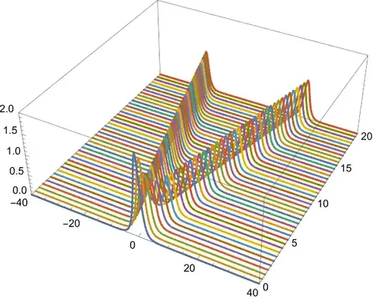
mat = Table[rs[[1]], {t, 0, 20, 0.5}];
ListLinePlot3D[Chop@InverseFourier[#, FourierParameters -> {-1, 1}] & /@ mat, 
 PlotRange -> All, DataRange -> {{-L/2, L/2}, {0, 20}}]

The code above can of course be simplified, but I'm too lazy to continue. Let me end this answer with a fully NDSolve-based solution for the problem as comparison:

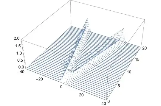
sys = With[{u = u[t, x]}, 
           {D[u, t, t] == a^2  D[u, x, x], 
           {u == 2 Sech[x], D[u, t] == 0} /. t -> 0, 
            (u /. x -> -L/2) == (u /. x -> L/2)}]
sol = NDSolveValue[sys, u, {t, 0, 20}, {x, -L/2, L/2}]
Plot3D[sol[t, x], {t, 0, 20}, {x, -L/2, L/2}, PlotRange -> All, PlotPoints -> 100]

---

Update

…If you insist on solving the problem based on the same logic as that of MATLAB, then we need a solver similar to ode45 i.e. an ODE solver taking the right hand side of ODE in standard form as the input. Luckily I've already written one here. Let's use it:

L = 80;
N0 = 256;
x = (L Range[-(N0/2), N0/2 - 1])/N0;
k = (2  π )/L Join[Range[0, N0/2 - 1], Range[-(N0/2), -1]];
u = 2 Sech[x];
ut = Fourier[u];
vt = ConstantArray[0, N0];
uvt = Join[ut, vt];
a = 1;
t0 = 0;
tend = 20;    
dt = 1/20;
t = Range[t0, tend, dt];
wave1D = With[{n = N0, a = a, k = k}, 
   Function[{t, uvt}, 
    Module[{ut, vt}, {ut, vt} = Partition[uvt, n]; Join[vt, -a^2  k^2  ut]]]];
(* Definition of rk4stepfunc is not included in this post,
   please find it in the link above. *)
step = (rk4stepfunc /. (Verbatim[_Real]) :> (_Complex))@wave1D;
solmat = FoldList[step[#2[[1]], #, #2[[2]]] &, uvt, 
    Transpose@{Most@t, Differences@t}]; // AbsoluteTiming
ListDensityPlot[Chop[InverseFourier /@ solmat[[;; ;; 10, 1 ;; N0]]], 
 DataRange -> {{-L/2, L/2}, {t0, tend}}, PlotRange -> All]

---

Update 2

If what you want is to convert the wave1D to Mathematica code and use it in NDSolve, define a black-box function. I'll show a somewhat advanced way for defining it just for fun:

L = 80;
N0 = 256;
x = (L Range[-N0/2, N0/2 - 1])/N0;
k = 2 π/L Join[Range[0, N0/2 - 1], Range[-N0/2, -1]];
u = 2 Sech[x];
ut = Fourier[u];
vt = ConstantArray[0, N0];
uvt = Join[ut, vt];
a = 1;
t0 = 0;
tend = 20;
wave1Dcompiled = 
 With[{n = N0, a = a, k = k}, 
  Compile[{t, {uvt, _Complex, 1}}, 
   Module[{ut, vt}, {ut, vt} = Partition[uvt, n]; Join[vt, -a^2  k^2  ut]], 
   RuntimeOptions -> EvaluateSymbolically -> False]]
solmat = NDSolveValue[{vec'[t] == wave1Dcompiled[t, vec[t]], vec[0] == uvt}, 
    vec /@ Range[0, tend, 1/2], {t, 0, tend}]; // AbsoluteTiming
ListPointPlot3D[Chop[InverseFourier /@ solmat[[All, ;; N0]]], PlotRange -> All, 
 DataRange -> {{-L/2, L/2}, {t0, tend}}]

Answer 2

I want to give a more concise code form by learning other people's answers. The original differential equation is not reduced in order.

Definition of fftshift is from the following post:

What's the correct way to shift zero frequency to the center of a Fourier Transform?

L = 80;
N0 = 256;
x = L/N0*Range[-N0/2, N0/2 - 1];
k = (2*Pi/L)*fftshift@Range[-N0/2, N0/2 - 1];
u = 2*Sech[x];
ut = Fourier[u, FourierParameters -> {-1, 1}];
a = 1;
U[t_] := Table[uf[i][t], {i, 1, N0}];
int1 = U[0] == ut;
int2 = U'[0] == ConstantArray[0, N0];
eqs = U''[t] == -a^2 k^2 U[t];
rs = NDSolveValue[{eqs, int1, int2}, U[t], {t, 0, 20}];
mat = Table[rs, {t, 0, 20, 0.5}]
ListLinePlot3D[
 Chop@InverseFourier[#, FourierParameters -> {-1, 1}] & /@ mat, 
 PlotRange -> All, DataRange -> {{-L/2, L/2}, {0, 20}}]