I have a complex function F[x,y], and now I want to plot the contour F[x,y] = 0. What can I do in order to have the contour plot vs Re[x] and y (That is, I want to treat y a real variable and x a complex one)?
Thanks you very much!
I have a complex function F[x,y], and now I want to plot the contour F[x,y] = 0. What can I do in order to have the contour plot vs Re[x] and y (That is, I want to treat y a real variable and x a complex one)?
Thanks you very much!
Let me make sure I understand your question correctly, taking your comments into account. You have a function $f:\mathbb C\times\mathbb C\to\mathbb C$. You want to plot the set of points $(a,b)\in\mathbb R^2$ such that $f(a+ic,b+0i)=0$ for some $c\in\mathbb R$. Right? Let me know if I've misinterpreted your question.
Aside: The entire zero set of $f$, the set of all points $(x,y)\in\mathbb C^2$ such that $f(x,y)=0$, can be interpreted geometrically as a two-dimensional real surface embedded in four-dimensional real space $\mathbb C^2\cong\mathbb R^4$. Your desired plot amounts to slicing the surface along $\operatorname{Im}y=0$, and projecting it under $x\mapsto\operatorname{Re}x$, to get a one-dimensional curve in $\mathbb R^2$ (corresponding to $(\operatorname{Re}x,\operatorname{Re}y)$).
Here's one way to do this. We have three real degrees of freedom, $a$, $b$, and $c$, with $x=a+ic$ and $y=b+0i$. The contour $f(x,y)=0$ is a curve in three-dimensional $(a,b,c)$ space, defined implicitly by two real equations $\operatorname{Re}f(x,y)=0$ and $\operatorname{Im}f(x,y)=0$. Fortunately there are very elegant ways to plot such a curve.
f[x_, y_] := x^2 + y^2 - 1

With[{x = a + I c, y = b + 0 I},
 ContourPlot3D[{Re@f[x, y], Im@f[x, y]},
  {a, -2, 2}, {b, -2, 2}, {c, -2, 2}, Contours -> {0}, Mesh -> None,
  ContourStyle -> {Directive[Lighter@Lighter@Blue, Opacity[0.4]],
    Directive[Lighter@Lighter@Red, Opacity[0.4]]},
  BoundaryStyle -> {1 -> None, 2 -> None, {1, 2} -> ColorData[1, 1]},
  PlotPoints -> 50, MaxRecursion -> 0]]

Aside: I used Maxim Rytin's method in Daniel Lichtblau's answer because Szabolcs's method draws extraneous curves at the plot boundaries. Also, for some reason the contours seem to get broken up if
MaxRecursionis nonzero.
Now we can rid of the $c$ coordinate in the plot just by looking at it from an orthogonal top-down view. But there is another problem: we have to set a finite range for $c$ in the plot, but there might be points on the curve which require arbitrarily large values of $c$. No problem! We'll let $c=g(t)$ for some function $g$ which maps a finite range to all of $\mathbb R$, and plot against $t$ instead. I like to use the logit function for this purpose, but you could use $\tan$, $\tanh^{-1}$, or anything like that.
With[{x = a + I (Log[t] - Log[1 - t]), y = b + 0 I},
 ContourPlot3D[{Re@f[x, y], Im@f[x, y]},
  {a, -2, 2}, {b, -2, 2}, {t, 0, 1}, Contours -> {0}, Mesh -> None, ContourStyle -> None,
  BoundaryStyle -> {1 -> None, 2 -> None, {1, 2} -> ColorData[1, 1]},
  ViewPoint -> {0, 0, Infinity}, PlotPoints -> 50, MaxRecursion -> 0]]

NSolve, which tries to find all the solutions. If that doesn't work, you could try posting a new question.
–
Aug 08 '13 at 20:38
What about the following:
F[x_, y_] := Sin[Sin[x - y]] + I Cos[Cos[x + y]];

With[{x = a - 3 I},
 ContourPlot[{Re[F[x, y]] == 0, Im[F[x, y]] == 0}, {a, -1, 1},
  {y, -3/2, 3/2}, FrameLabel -> (Text[Style[#, Italic, 16]] & /@ {"Re x", "y"})]
]
which produces
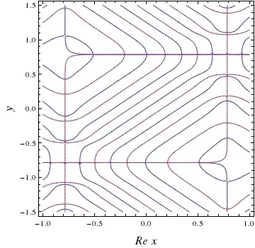
Im[x], I've assumed this to sketch this example.
– mmal
Aug 02 '13 at 12:15