6

I have the following Mathematica code:

f[r_] := 
 1 + r^2/(
   2 α) (1 - Sqrt[1 + 4 α ((2 M)/r^3 - q^2/r^4 - 1/l^2)])

M = rh/2 + q^2/(2 rh) + rh^3/(2 l^2) + α/(2 rh);

T[rh_] := (rh^2 - q^2 - α + 3 rh^4 l^-2)/( 4 π rh (rh^2 + 2 α))

V[r_] := f[r] (En^2/f[r] + L^2/r^2 + 1)

q = 0.02; α = 0.0065; l = 1; En = 0; L = 20;

rhmin = SolveValues[T[rh] == 0, rh, Reals][[2]]

Plot3D[V[r], {rh, rhmin, 1}, {r, rh, 5}, PlotRange -> All, PlotPoints -> 100]

which gives me the following 3DPlot:

3dplot

Now I find the stationary points of $V(r)$, which include both the local maxima and minima:

rsolmax[rh_] = SolveValues[{V'[r] == 0, V''[r] < 0}, r][[{3, 4, 5}]];

rsolmin[rh_] = SolveValues[{V'[r] == 0, V''[r] > 0}, r][[{6, 7}]];

and get this 2D plot:

Plot[Evaluate[{rsolmax[rh], rsolmin[rh]}], {rh, rhmin, 0.8776235}]

2dplot

Now I wish to project this plot of stationary points just below the 3DPlot, which should look something like this:

paper

How to get the desired result? Any help in this regard would be truly beneficial!

E. Chan-López
  • 23,117
  • 3
  • 21
  • 44
codebpr
  • 2,233
  • 1
  • 7
  • 26

3 Answers3

9

Use ContourPlot or ContourPlot3D to draw V'[r]==0 and set the range of z to {z, -800, -1000}.

We use V''[r] as the mesh shading functions and set Mesh->{{0}} to determinate where V''[r]>0 and V''[r]<0.

Clear[plot, belt]; plot = 
 Plot3D[V[r], {rh, rhmin, 1}, {r, rh, 5}, PlotRange -> All, 
  PlotPoints -> 50, 
  ColorFunction -> Function[{rh, r, z}, Blend[{LightBlue, Blue}, z]], 
  PlotTheme -> "Scientific", AxesLabel -> {rh, r, V}];
belt = ContourPlot3D[
   V'[r] == 0, {rh, rhmin, 1}, {r, rh, 5}, {z, -800, -1000}, 
   PlotRange -> All, MeshFunctions -> Function[{rh, r, z}, V''[r]], 
   Mesh -> {{0}}, MeshShading -> {Green, Pink}];
Show[plot, belt, Lighting -> {{"Ambient", White}}, 
 BoxRatios -> {1, 1, 1}, ViewPoint -> {0.95, -3.16, 0.56}]

enter image description here

herbertfederer
  • 1,180
  • 4
  • 13
  • That's a clever answer. I get similar results when I increase PlotPoints in the Contour Plot. Just one doubt, how can I choose my colour function to distinguish between the local maxima and the minima? – codebpr Feb 06 '24 at 14:58
8

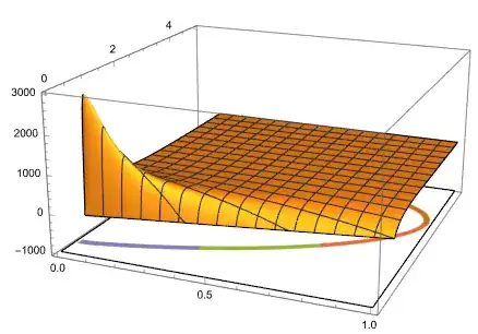
Perhaps this is a starting point (assuming the OP code):

f[x_, y_] := V'[y] /. rh -> x
p = Plot3D[V[r], {rh, rhmin, 1}, {r, rh, 5}, PlotRange -> All, 
  PlotPoints -> 100, MeshFunctions -> (f[#1, #2] &), Mesh -> {{0}}]

Projection:

pts = p[[1, 1, 1]];
i = Cases[p, Line[x_] :> x, Infinity][[2]];
crit = {#1, #2, -10000} & @@@ pts[[i]];
Show[p, Graphics3D[Line[crit]]]

enter image description here

ubpdqn
  • 60,617
  • 3
  • 59
  • 148
7

You may achieve a projection using Texture. A nice example can be found in: 2D projection of a 3D surface

tex = Plot[
   Evaluate[{rsolmax[rh], rsolmin[rh]}], {rh, rhmin, 0.8776235}, 
   PlotStyle -> Thickness[0.02], Axes -> False];
Graphics3D[{First[pl], Texture[tex], 
  Polygon[{{0, 0, -1000}, {1, 0, -1000}, {1, 5, -1000}, {0, 
     5, -1000}}, 
   VertexTextureCoordinates -> {{0, 0}, {1, 0}, {1, 1}, {0, 1}}]}, 
 BoxRatios -> {1, 1, 1/2}, Lighting -> "Neutral", Axes -> True]

enter image description here

Daniel Huber
  • 51,463
  • 1
  • 23
  • 57