Plotting a Phase Portrait of an ODE

Question

I'm trying to get a Mathematica program to plot a phase portrait of this differential equation:

$$\frac{dv}{dt} = g - \frac{k}{m}v^2$$

where g, k, m are physical constants. I want to make it such that the x axis is time t and y axis is velocity v(t). How do I use VectorPlot or StreamPlot to accomplish this?

Answer 1

I've checked all of those; I am not quite sure if any of them have the time as the x-axis

The syntax to generate phase plot for first order ode of form $$ y'(x) = \frac{A(x,y)}{B(x,y)} $$

is

StreamPlot[{B,A},{x,from,to},{y,from,to}]

So using the above on your ode, where now y is your v and x is your t gives

\begin{align*} \frac{dv}{dt} &= g - \frac{k}{m}v^2\\ &= \frac{g - \frac{k}{m}v^2}{1} \end{align*}

Hence setting some values for g and m and k gives

g = 9.81; m = 10; k = 0.1;
StreamPlot[{1, g - k/m*v^2}, {t, 0, 10}, {v, -10, 10}, 
 FrameLabel -> {"t", "v(t)"}, BaseStyle -> 20]

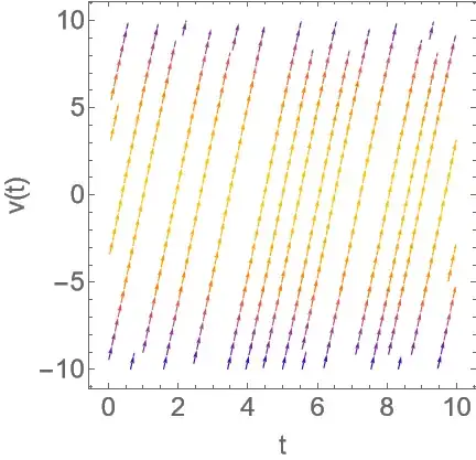
The above shows solutions curves. If you have a specific IC, then one of these curves will be the solution.

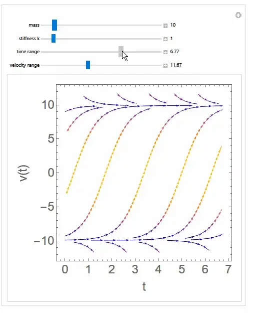
Here is a Manipulate to make it easier to analyze the system

Manipulate[
 Module[{g = 9.81},
  StreamPlot[{1, g - k/m*v^2}, {t, 0, maxtime}, {v, -maxV, maxV}, 
   FrameLabel -> {"t", "v(t)"}, BaseStyle -> 20]
  ]
 ,
 {{m, 10, "mass"}, 0.1, 100, .1, Appearance -> "Labeled"},
 {{k, 1, "stiffness k"}, 0.1, 10, .1, Appearance -> "Labeled"},
 {{maxtime, 1, "time range"}, 0.01, 10, .01, 
  Appearance -> "Labeled"},
 {{maxV, 1, "velocity range"}, 0.01, 30, .01, Appearance -> "Labeled"},
 TrackedSymbols :> {m, k, maxtime, maxV}
 ]