I'm trying to plot a phase portrait for the differential equation $$x'' - (1 - x^2) x' + x = 0.5 \cos(1.1 t)\,.$$ The primes are derivatives with respect to $t$. I've reduced this second order ODE to two first order ODEs of the form $ x_1' = x_2$ and $x_2' - (1 - x_1^2) x_2 + x_1 = 0.5 \cos(1.1 t)$. Now I wish to use mathematica to plot a phase portrait. Unfortunately, I'm unsure of how to do this because of the dependence of the second equation on an explicit $t$.
Asked
Active
Viewed 7.2k times
46
3 Answers
47
again just a slight modification from the documentation
splot = StreamPlot[{y, (1 - x^2) y - x}, {x, -4, 4}, {y, -3, 3},
   StreamColorFunction -> "Rainbow"];
Manipulate[
 Show[splot,
  ParametricPlot[
   Evaluate[
    First[{x[t], y[t]} /.
      NDSolve[{x'[t] == y[t],
        y'[t] == y[t] (1 - x[t]^2) - x[t] + 0.5 Cos[1.1 t],
        Thread[{x[0], y[0]} == point]}, {x, y}, {t, 0, T}]]], {t, 0,
    T}, PlotStyle -> Red]], {{T, 20}, 1, 100}, {{point, {3, 0}},
  Locator}, SaveDefinitions -> True]

Or just to show off (again a rip off from the documentation)
splot = LineIntegralConvolutionPlot[{{y, (1 - x^2) y - x}, {"noise",
     1000, 1000}}, {x, -4, 4}, {y, -3, 3},
   ColorFunction -> "BeachColors", LightingAngle -> 0,
   LineIntegralConvolutionScale -> 3, Frame -> False];
Manipulate[
 Show[splot,
  ParametricPlot[
   Evaluate[
    First[{x[t], y[t]} /.
      NDSolve[{x'[t] == y[t], y'[t] == y[t] (1 - x[t]^2) - x[t]+0.5 Cos[1.1 t],
        Thread[{x[0], y[0]} == point]}, {x, y}, {t, 0, T}]]], {t, 0,
    T}, PlotStyle -> White]], {{T, 20}, 1, 100}, {{point, {3, 0}},
  Locator}, SaveDefinitions -> True]

chris
- 22,860
- 5
- 60
- 149
-
Just a question. Is it right, that StreamPlot[{v1[x,y],v2[x,y]}] returns a set of solutions of the differential equations x'=v1; y'=v2? It looks like an elementary information that everybody knows. But it happened that I do not know, and there is no explicit discussion of this point in the Help/StreamPlot. Please let me know. Where could I have a look at the proof, or at least, an explanation? If I understand right, the StreamPlot simply yields the phase portrait, does it? – Alexei Boulbitch Nov 06 '12 at 10:51
-
@AlexeiBoulbitch yes it yields a set of solutions for the homogenous set of equations. But it does not attempt to be continuous. In the previous example if you remove
+ 0.5 Cos[1.1 t]you will see that the red curve and the underlying flow become identical. – chris Nov 07 '12 at 17:48
42
The EquationTrekker package is a great package for plotting and exploring phase space
<< EquationTrekker`
EquationTrekker[x''[t] - (1 - x[t]^2) x'[t] + x[t] == 0.5 Cos[1.1 t], x[t], {t, 0, 10}]
This brings up a window where you can right click on any point and it plots the trajectory starting with that initial condition:

You can do more as well, such as add parameters to your equations and see what happens to the trajectories as you vary them:
 EquationTrekker[x''[t] - (1 - x[t]^2) x'[t] + x[t] == a Cos[\[Omega] t],
                 x[t], {t, 0, 10}, TrekParameters -> {a -> 0.5, \[Omega] -> 1.1}
                ]

David Slater
- 1,525
- 10
- 13
-
3This no longer works in the version I have, 11.0.0.0. It produces error messages and no output. This is what has happened every time I've tried a Mathematica package. They always seem to fail in the version I am using. Sometimes I can fix the resulting errors, but usually not. In the end I always have to go back to built-in functionality, which seldom fails in my experience. – Ralph Dratman Apr 04 '17 at 23:36
-
Hi, this package has a large number of errors in version 12.1 and cannot be used. – A little mouse on the pampas Jul 24 '20 at 01:01
-
1See https://mathematica.stackexchange.com/questions/92810/equationtrekker-using-mathematica-10-2 for more about how to use EquationTrekker in versions since V10.2 – Michael E2 Nov 01 '20 at 00:40
26
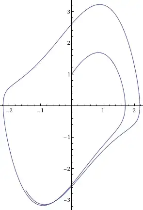
You can solve the equation with (you might want to change the initial conditions) :
sol[t_] =  NDSolve[{x''[t] - (1 - x[t]^2) x'[t] + x[t] == 0.5 Cos[1.1 t],
   x[0] == 0, x'[0] == 1}, x[t], {t, 0, 10}][[1, 1, 2]]
Now you can use the solution as any other function; in particular, you can plot it versus its derivative :
ParametricPlot[{sol[t], sol'[t]}, {t, 0, 10}]
b.gates.you.know.what
- 20,103
- 2
- 43
- 84
ParametricPlot. – b.gates.you.know.what Nov 05 '12 at 18:42NDSolve,ParametricPlot,StreamPlot, etc.) Just the first two should be sufficient for you to make headway on your problem. – rm -rf Nov 05 '12 at 18:55