Solve polynomial functions with four unknown variables

Question

I want to make curve with polynominal function like this figure

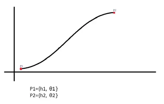
but only 2 known point to solve this one. I try to used solve function for this one. but the result is not the same like the figure.

here is my code

h1 = 50;
h2 = 80;
[Theta]1 = 5 [Pi];
[Theta]2 = 9 [Pi];
eq1 = a0 + (a1[Theta]1) + (a2[Theta]1^2) + (a3[Theta]1^3) == 
   h1;
eq2 = a1 + (a2[Theta]1) + (a3[Theta]1^2) == 0;
eq3 = a0 + (a1[Theta]2) + (a2[Theta]2^2) + (a3[Theta]2^3) == 
   h2;
eq4 = a1 + (a2[Theta]2) + (a3[Theta]2^2) == 0;
va = NSolve[{eq1, eq2, eq3, eq4}, {a0, a1, a2, a3}, Reals, 
   WorkingPrecision -> 7];
eq = (a0 + a1 # + a2 #^2 + a3 #^3) &;
P = eq[t] /. va[[1]] // N
Plot[P, {t, [Theta]1, [Theta]2}]

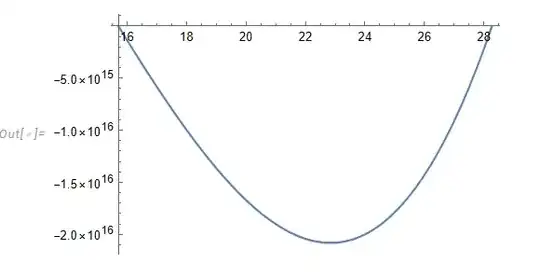
this is my curve result with that code

Thank you everyone

Your problem is underdefined. There are infinitely many polynomials that go through those two points. The simplest is just a straight line. — ScienceSnake, Mar 09 '24 at 12:45
Hard to tell if it is. Look at the y axis, you're so zoomed out it's impossible to see anything. — ScienceSnake, Mar 09 '24 at 13:18
The way to go is described here: Get polynomial interpolation formula. — Artes, Mar 09 '24 at 13:19

score 2 · Accepted Answer · answered Mar 09 '24 at 13:49

I'm assuming what the OP wants is the lowest order polynomial that goes through two given points and has 0 gradient at those two points. The latter isn't explicitly stated, but I implied it from the diagram and the use of a cubic polynomial.

For this problem, we have 4 constraints, and therefore require a polynomial with 4 coefficients, aka, a cubic. This can then be passed to solved along with the constraints and plotted, giving a graph similar to what was in the question:

h1 = 50;
h2 = 80;
\[Theta]1 = 5 \[Pi];
\[Theta]2 = 9 \[Pi];
f[[Theta]_]:= a [Theta]^3+b [Theta]^2 + c [Theta] + d
sols = Solve[{f[[Theta]1] == h1, f[[Theta]2]==h2, f'[[Theta]1]==f'[[Theta]2]==0},
             {a, b, c, d}];
fSolve[[Theta]_] = f[[Theta]] /. sols[[1]]
Show[
  Plot[fSolve[[Theta]], {[Theta], [Theta]1, [Theta]2},
      PlotRange->{{[Theta]1-[Pi], [Theta]2+[Pi]}, {h1-10, h2+10}}],
    Graphics[{PointSize[Large], Red, Point[{[Theta]1, h1}]}],
    Graphics[{PointSize[Large], Red, Point[{[Theta]2, h2}]}]
]
out = 4925/16-(2025 [Theta])/(16 [Pi])+(315 [Theta]^2)/(16 [Pi]^2)-(15 [Theta]^3)/(16 [Pi]^3)

wow, nice, that what I want! thank you for your help – 葉柏樂 Mar 11 '24 at 05:53 — 葉柏樂, Mar 11 '24 at 05:53

Solve polynomial functions with four unknown variables

1 Answers1