Get polynomial interpolation formula

Question

I'm attempting to get a polynomial interpolation formula out of Mathematica but I am absolutely lost. I stared out using Wolfram|Alpha, but it seems as if my input had become too large.

I tried using this on WolframAlpha.com :

Interpolate {1,33},{2,80},{5,286},{10,771},{15,1382},{20,2087},{25,2867},{30,3707},{40,5526},
{50,7470},{60,9482},{70,11507},{80,13495},{90,15391},{100,17313},{110,18631},{120,19752},
{125,20064}

but I get an error.

Thinking that Mathematica was the solution I signed up for a trial but I can't seem to get an interpolation formula out of it. Searching Google and this exchange has given me very few results.

Any idea how I can just get a polynomial interpolation formula from my dataset?

Answer 1

You may want a quick sketch :)

Or, you could also solve the Vandermonde matrix:

n = 10;(* points number*)
{xi, yi} = RandomReal[{0, 1}, {2, n}];
a = LinearSolve[Transpose@Table[xi^k, {k, 0, n - 1}], yi]

(* System solved, now plot it *)
p[x_, m_] := Sum[a[[i + 1]] x^i, {i, 0, m}];
Show[Plot[p[x, n - 1], {x, 0, 1},  PlotRange -> {Automatic, {-20, 20}}], 
     ListPlot[Transpose[{xi, yi}], PlotStyle -> {PointSize[Medium], Red}]]

Just be aware that it may, depending on your points, results in an ill-conditioned system

Answer 2

First take your data

data = {{1, 33}, {2, 80}, {5, 286}, {10, 771}, {15, 1382}, {20, 
2087}, {25, 2867}, {30, 3707}, {40, 5526}, {50, 7470}, {60, 
9482}, {70, 11507}, {80, 13495}, {90, 15391}, {100, 17313}, {110, 
18631}, {120, 19752}, {125, 20064}};

Then we call LinearModelFit and fit a cubic polynomial to your data.

lm = LinearModelFit[data, {x^3, x^2, x}, x];
Show[ListPlot[data, PlotStyle -> Red,Filling->Bottom],Plot[lm[x],{x, 0, 125}],Frame -> True]

And to get the polynomial that best fits your data.

Normal[lm]

-83.6419 + 69.7325 x + 2.19787 x^2 - 0.0116981 x^3

Now you must realize that above polynomial is not an interpolation of your data but a best continuous approximation of it with respect to the Euclidean norm. Forming a interpolating polynomial for a data of $n$ points require at least a $n$-th degree polynomial. This is not practical as higher degree polynomials come with higher and unwanted oscillations. Hence people use polynomials for peace-wise interpolation. HermitePolynomil can be used for this purpose.

But if you want you can get an interpolating polynomial for your data as follows.

InterpolatingPolynomial[data, x] // Expand // N

3.1289 + 18.9719 x + 12.41 x^2 - 1.71825 x^3 + 0.228052 x^4 - 0.0219672 x^5 + 0.00150955 x^6 - 0.0000751269 x^7 + 2.75112*10^-6 x^8 - 7.49912*10^-8 x^9 + 1.53098*10^-9 x^10 - 2.34119*10^-11 x^11 + 2.66291*10^-13 x^12 - 2.216*10^-15 x^13 + 1.30841*10^-17 x^14 - 5.18423*10^-20 x^15 + 1.2348*10^-22 x^16 - 1.33508*10^-25 x^17

You can see the above polynomial has degree 17 and you have 18 data entries. This interpolating polynomial also fails to keep up with the data trend. You can see this phenomena in the boundaries of the following plot. For $x$ outside your data range the mammoth polynomial (dashed one) starts to disagree with given data trend almost exponentially! The approximating cubic polynomial (thick red one) captures the data behavior very well even beyond the given data range.

Answer 3

Evaluating what the OP tried with free-form input (shortcut =) yields a suggestion cell with this input : Expand[ InterpolatingPolynomial[{286, 771}, x]], similarly a Wolfram|Alpha query yields input interpretation interpolating polynomial, so it is not especially difficult to surmise that the desired function is InterpolatingPolynomial. Defining the list l :

l = {{1, 33}, {2, 80}, {5, 286}, {10, 771}, {15, 1382}, {20, 2087}, {25, 2867}, {30, 3707},
     {40, 5526}, {50, 7470}, {60, 9482}, {70, 11507}, {80, 13495}, {90, 15391}, {100, 17313},
     {110, 18631}, {120, 19752}, {125, 20064}};

the resulting polynomial (written in a standard expanded form ) is :

p[x_] := Expand @ InterpolatingPolynomial[ l, x]

How could we define an interpolating polynomial having no InterpolatingPolynomial built-in function ?

A natural way is to define recursively a family of polynomials. In order to make it possibly fast we can take advantage of memoization techiques (see e.g. answers to What is “x := x =” trickery? or Why does Expand not work within a function? )

poly[x_, 0]  := l[[1, 2]]
poly[x_, k_] := poly[ x, k] = poly[ x, k-1] + 
               (l[[k, 2]] - poly[l[[k, 1]], k-1]) Product[(x-l[[j, 1]])/(l[[k, 1]]-l[[j, 1]]),
                                                           {j, k - 1}]

let's check if it works properly :

Expand @ poly[ x, Length @ l] === p[x]

True

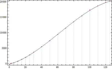
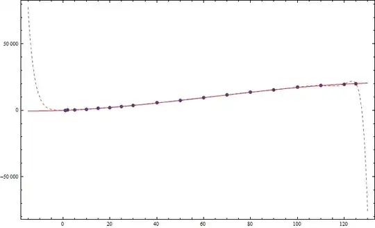
Well indeed, now we can imagine what is behind InterpolatingPolynomial so let's restrict to p[x] being a seventeenth order polynomial with rational coefficients (in general when the list is of length n then the polynomial will be of order n-1, and if l is a list of rational pairs, p will be a polynomial with rational coefficients). One can reproduce the list l with p[x] :

p[#] & /@ l[[All, 1]] == l[[All, 2]]

True

Since its coefficients are a bit involved we prefer to write them this way :

p[x] // TraditionalForm // N

Plot[ p[x], {x, -12, 128}, PlotStyle -> Thick, Epilog -> {Red, PointSize[0.01], Point[l]}]