Plotting an epicycloid

Question

I am fairly new to Mathematica, and I cannot figure out how to plot an epicycloid. I have plotted some neat looking things in my attempts, but I still can't make one. I am not looking to make an animation; I just want the plot of an epicycloid.

Would I use PolarPlot or ParametricPlot? How do I get a static picture of an epicycloid?

Welcome to Mathematica.SE! Have a look at http://demonstrations.wolfram.com/search.html?query=epicycloid — Yves Klett, Sep 16 '13 at 14:56
Mostly a lot of fiddling with the epicycloid equations in a PolarPlot (and some ParametricPlots). — btalbot, Sep 16 '13 at 14:56
@PinguinDirk is asking you to post the code you have tried thus far, so we can see where there might be a problem. — bobthechemist, Sep 16 '13 at 15:20

C. E. · Accepted Answer · 2016-07-23T20:02:38.773

38

I recreated the animation on Wikipedia:

enter image description here

Here is the Manipulate version:

R = 3; r = 1;

fx[θ_, a_: 1] := (R + r) Cos[θ] - a r Cos[(R + r) θ/r];
fy[θ_, a_: 1] := (R + r) Sin[θ] - a r Sin[(R + r) θ/r];

gridlines = Table[{x, GrayLevel[0.9]}, {x, -6, 6, 0.5}];

plot[max_] := ParametricPlot[
  {fx[θ], fy[θ]}, {θ, 0, max},
  PlotStyle -> {Red, Thick},
  Epilog -> {
    Thick,
    Blue, Circle[{0, 0}, R],
    Black, Circle[{fx[max, 0], fy[max, 0]}, r],
    Red, PointSize[Large], Point[{fx[max], fy[max]}],
    Black, Line[{{fx[max, 0], fy[max, 0]}, {fx[max], fy[max]}}]
    },
  GridLines -> {gridlines, gridlines},
  PlotRange -> {-6, 6}
  ]
Manipulate[plot[max], {max, 0.01, 2 Pi}]

edited Jul 23 '16 at 20:02

answered Sep 16 '13 at 19:02

C. E.

70,533
6
140
264

3

I don't know how many hours I've spent (wasted) on playing with roulettes, but it sure was fun. :) – J. M.'s missing motivation May 03 '15 at 06:54
@J.M. Upvote for that masterpiece. :) – yode Jul 24 '16 at 06:52

kirma · Answer 2 · 2013-09-16T18:48:56.557

18

It is easiest to use ParametricPlot and RotationTransform.

ParametricPlot[
  RotationTransform[a][{1, 0}] + RotationTransform[4 a][{1/4, 0}],
  {a, 0, 2 Pi}, Evaluated -> True]

Evaluated -> True is not strictly necessary; it's there just to construct the equation once instead of for every point in the graph separately (... which is slow).

EDIT: Improved per comment from Mr.Wizard.

edited Sep 16 '13 at 18:48

answered Sep 16 '13 at 15:10

kirma

19,056
1
51
93

2

+1 -- however, I recommend using the Evaluated -> True option rather than Evaluate to properly localize a. Please see: (7832), (5220), (7561) – Mr.Wizard Sep 16 '13 at 17:34

score 17 · Answer 3 · edited Jun 16 '20 at 09:23

Epicycloids (and other roulette curves) are fun to play with using Manipulate. Here is one of many possible implementations.

Manipulate[
  ParametricPlot[{
    (1 + r)  Cos[theta] + a Cos[(1 + r) theta], 
    (1 + r) Sin[theta] + a Sin[(1 + r) theta]}, 
    {theta, 0, 2 Pi}],
  {{r, 1}, 1, 20, 1, Appearance -> "Labeled"},
  {{a, 1}, -10, 10, .2, Appearance -> "Labeled"}]

Edit

Although the question only calls for epicycloids, it is very easy to make interactive panel that allows the user to play with hypocycloids as well. Because there is a simple relationship between epicycloids and hypocycloids, doing so adds very little code.

Manipulate[
  ParametricPlot[{
      type r Cos[theta] + a Cos[type r theta], 
      type r Sin[theta] + a Sin[type  r theta]},
    {theta, 0, 2 Pi},
    PlotStyle -> {Red, Thick},
    ImageSize -> {400, 400}],
  {{type, 1}, {1 -> "epicycloid", -1 -> "hypocycloid"}},
  {{r, 1}, 1, 20, 1, Appearance -> "Labeled"},
  {{a, 1}, -10, 10, .1, Appearance -> "Labeled"}]

score 13 · Answer 4 · answered Sep 16 '13 at 16:57

Looking up epicycloid we get the parametric equations describing it and then ParametricPlot does the rest of our work.

ParametricPlot[
     {3 3.1 Cos[θ] - 3 Cos[3.1 θ], 3 3.1 Sin[θ] - 3 Sin[3.1 θ]}, 
     {θ, 0, 20 π},
     ColorFunction -> "AtlanticColors"]

J. M.'s missing motivation · Answer 5 · 2016-07-23T19:28:10.603

Just for fun, here is a variation of C. E.'s animation, which demonstrates that an epicycloid can be constructed as an envelope of the diameter of a rolling circle:

With[{n = 3, r = 1, m = 31},
     Animate[ParametricPlot[ReIm[(n + 1) r E^(I t) - r E^(I (n + 1) t)],
                            {t, 0, 2 Denominator[n] π}, Axes -> None, 
                            Epilog -> {Circle[ReIm[(n + 2) r E^(I u)], 2 r],
                                       {Red, Line[{ReIm[(n + 2) r E^(I u) -
                                                        2 r E^(I (1 + n/2) u)], 
                                                   ReIm[(n + 2) r E^(I u) +
                                                        2 r E^(I (1 + n/2) u)]}]}}, 
                            Frame -> True, PlotRange -> (n + 4) r, 
                            PlotStyle -> Red, Prolog -> {Blue, Circle[{0, 0}, n r]}],
             {u, 0, 2 Denominator[n] π, (2 Denominator[n] π)/(m - 1)}]]

epicycloid as envelope

(Note the use of the complex form of the epicycloid.)

A slight modification of the code given above can be done to produce the multiple exposure version:

If one just wants to see the lines enveloping the epicycloid, the code is much simpler:

With[{n = 3, r = 1, m = 101}, 
     Graphics[{Opacity[1/5], 
               Table[InfiniteLine[{ReIm[(n + 2) r E^(I u) - 2 r E^(I (1 + n/2) u)], 
                                   ReIm[(n + 2) r E^(I u) + 2 r E^(I (1 + n/2) u)]}],
                     {u, 0, 2 Denominator[n] π, (2 Denominator[n] π)/(m - 1)}]}]]

just the envelope please, Louise

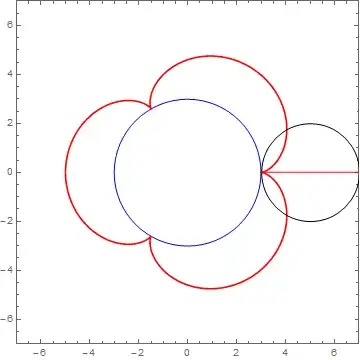
Still another neat demonstration is the Bernoulli-Euler double generation theorem: an epicycloid is equivalent to a pericycloid (which can be thought of as the locus of a point mounted on a "hula hoop").

With[{n = 3, r = 1, m = 31},
     Animate[{ParametricPlot[ReIm[(n + 1) r E^(I t) - r E^(I (n + 1) t)],
                             {t, -$MachineEpsilon, u}, Axes -> None, 
                             Epilog -> {Thick, Circle[ReIm[(n + 1) r E^(I u)], r], 
                                        Line[{ReIm[(n + 1) r E^(I u)], 
                                              ReIm[(n + 1) r E^(I u) -
                                                   r E^(I (n + 1) u)]}],
                                        {Directive[Red, PointSize[Large]], 
                                         Point[ReIm[(n + 1) r E^(I u) -
                                                    r E^(I (n + 1) u)]]}}, 
                             Frame -> True, PlotRange -> (n + 2) r, 
                             PlotStyle -> Directive[Red, Thick], 
                             Prolog -> {Directive[Blue, Thick], Circle[{0, 0}, n r]}], 
              ParametricPlot[ReIm[(n + 1) r E^(I t) - r E^(I (n + 1) t)],
                             {t, -$MachineEpsilon, u}, Axes -> None, 
                             Epilog -> {Thick, Circle[ReIm[-r E^(I (n + 1) u)],
                                                      (n + 1) r], 
                                        Line[{ReIm[-r E^(I (n + 1) u)], 
                                              ReIm[(n + 1) r E^(I u) -
                                                   r E^(I (n + 1) u)]}],
                                        {Directive[Red, PointSize[Large]], 
                                         Point[ReIm[(n + 1) r E^(I u) -
                                                    r E^(I (n + 1) u)]]}}, 
                             Frame -> True, PlotRange -> (n + 2) r, 
                             PlotStyle -> Directive[Red, Thick], 
                             Prolog -> {Directive[Blue, Thick], Circle[{0, 0}, n r]}]}
             // GraphicsRow, {u, 0, 2 Denominator[n] π, (2 Denominator[n] π)/(m - 1)}]]

Plotting an epicycloid

5 Answers5

Edit

Linked