1

First I want to solve an equation $F(x,y)=0$ for $y$ by supplying a value of $x$. (suppose obtaining the analytic form of $y(x)$ is too difficult) Then I want to plot root $y$ (numerically calculated) as a function of $x$ by using the following:

Plot[y /. FindRoot[.../.{x->x0},{y, 0.2}],{x0, 0, 1}]

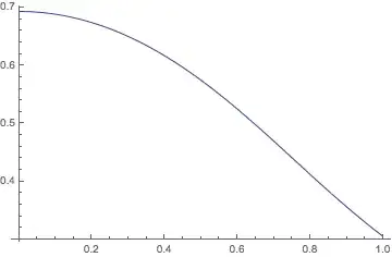
and I got something like the following

enter image description here

I omit ... here since it is terribly complicated. Update: F(x,y) is of the form

$\sum_{n,m}a_{m,n}x^ny^m$

and $m$ and $n$ can be as high as 19, which basically makes Solve impractical.

The result is satisfying except a small number of points near 1.0. Setting another initial starting value of $y$ in FindRoot might be an option but it is very tedious and often I cannot find a value of $y$ that fits the whole range of $x$.

My question is: suppose I stick with the initial value of $y$, is there a way to just eliminate that anomaly point after I Plot the numerical results? Or is there a better way to deal with this kind of numerical problem in general?

wdg
  • 1,189
  • 9
  • 18
  • For some functions you can use the previously found root to start looking for the next. But I can't know how your function behaves since it isn't supplied. – C. E. Oct 23 '13 at 07:58
  • @Anon,sounds like a good idea, could you write some code on it? For the function, it is rational function very similar to a Pade approximant. But it is too complicated to be readable so I didn't put it in the question. – wdg Oct 23 '13 at 08:13
  • 1
    @wdg You could try to use the form FindRoot[...,{x,xstart,xmin,xmax}] and restrict the search to [0,1]. Maybe this helps. – halirutan Oct 23 '13 at 08:16
  • @halirutan, it does help! – wdg Oct 23 '13 at 08:22

3 Answers3

2

In case it helps to determine the new initial search value from the old, which is sometimes the case, it can be done like this:

f[x_, y_] := ArcTan[x + y]
x0 = 0;
Plot[(x0 = FindRoot[f[x, y], {x, x0}][[1, 2]]), {y, -100, 100}]
C. E.
  • 70,533
  • 6
  • 140
  • 264
  • This method works well if the value of y is changing slowly from step to step, for example when creating a table of values for ListPlot. However, Plot will sample the function at y values which hop around all over the place as it goes through the recursive refinement process, so I don't think this method is reliable. – Simon Woods Oct 23 '13 at 09:00
  • @SimonWoods You are absolutely right! I stored the y-values in this example using Sow and the largest differences were very large which is not something I had anticipated. It's still better than using a static initial value, I think, but as you say it's better to use Table and ListPlot to do it this way. – C. E. Oct 23 '13 at 12:31
2

Like this:?

Here I give F(x,y)= Abs@x + Abs@(x + y)-1

Plot[y /. Solve[Abs@x + Abs@(x + y) == 1, y, Reals] // 
       Evaluate, {x, -2, 2}, AspectRatio -> Automatic]

enter image description here

Another methods:

Using the ContourPlot command

ContourPlot[Abs[x] + Abs[x + y] == 1, {x, -2, 2}, {y, -2, 2}, 
AxesOrigin -> {0, 0}, Frame -> False, Axes -> True]
xyz
  • 605
  • 4
  • 38
  • 117
  • ContourPlot is a good idea. In fact I often use ContourPlot to verify numerical results obtained through other means. – wdg Oct 23 '13 at 13:21
1

Using NDSolve to create an interpolation often works well. Hard to tell if it will work with your function.

With[{f = x^2 y + y^3 - 1/3},
 sol = NDSolveValue[{Dt[f == 0, x] /. y -> y[x], 
    y[0] == (y /. FindRoot[f /. x -> 0, {y, 0.6}])}, y, {x, 0, 1}]]
(* InterpolatingFunction[{{0., 1.}}, <>] *)

Plot[sol[x], {x, 0, 1}]

Mathematica graphics

Michael E2
  • 235,386
  • 17
  • 334
  • 747