There is a difficulty with the statement of the problem. Generally the problem can be solved as shown below. In this case there is a stipulation that $1 < x < 5$ and $1 < y < 5$. Unfortunately the solution to the system does not satisfy these constraints (also shown below).
If we agree to use only numerical techniques and pretend that Solve (nor NSolve) will not produce solutions, then FindRoot is the way to find a single solution. The best way to make an interpolating function for y as a function of x is via NDSolve and a differential-algebraic equation. Below I assume that the equations eqn1 and eqn2 actually define y as a unique function of x. In some systems, this will not be true, and one may have to do more work to determine which branch or branches are to be computed.
We have to find the first point of the intersection with FindRoot. The starting point {x, y, z} = {1, 1, 1} for FindRoot may have to be tweaked for other systems. (It's not a terribly enlightened guess for this specific case, either, but this case is easy for FindRoot.)
eqn1 = 3/(x y z) - 2 x - 3 y - 5 z == 3;
eqn2 = x + y + z == 0;

ic = FindRoot[eqn1 && eqn2 && x == 1, {x, 1}, {y, 1}, {z, 1}]  (* initial values for x, y, z *)

yIFN = NDSolveValue[
  {x'[t] ==  1, {x[1], y[1], z[1]} == ({x, y, z} /. ic),
   {eqn1, eqn2} /. v : (x | y | z) :> v[t]}, y, {t, 1, 5}]
(*
  {x -> 1., y -> 0.890705, z -> -1.8907}

  InterpolatingFunction[{{1., 5.}}, <>]
*)

Plot[yIFN[x], {x, 1, 5}]

Note that by the initial value problem given to NDSolve, x and t are the same.
Note also that 0 < y < 1 -- that is, it does not satisfy the constraint in the problem. Here is another view of the problem in x y z space:
Show[
 ContourPlot3D[
  Evaluate@{eqn1, eqn2}, {x, 0, 5}, {y, 0, 5}, {z, 0, -5},
  ContourStyle -> Opacity[0.5], AxesLabel -> Automatic],
 ParametricPlot3D[{x, yIFN[x], -x - yIFN[x]}, {x, 1, 5},
  PlotStyle -> {Red, Thickness[0.02]}],
 PlotRange -> All
 ]
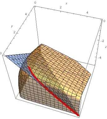
The intersection of the surfaces defined by eqn1 and eqn2 lies outside the region $1 < x < 5$, $1 < y < 5$.
Edit: On setting up NDSolve
To use NDSolveValue, I needed to change simple variables x, y, z to functions x[t], y[t], z[t]. One could simply retype them, but I tend to do it programmatically (if it's convenient -- as you get more familiar with a system, what seem convenient expands). This saves headaches on typos (for me at least) and updating changes to the equations.
Rules and Patterns (->, :>, etc. see What are the most common pitfalls awaiting new users? for a index of such signs) are fundamental objects. Function definitions are stored as rules in a functions DownValues. Many functions return them, such as FindRoot above. The first two links of this paragraph have tutorials and documentation pages for learning about these important objects.
The rules in ic replace the variables x, y, z by the coordinates of the point of intersection of the two surfaces eqn1, eqn2 with the plane x == 1 that was found by FindRoot:
{x'[t] == 1, {x[1], y[1], z[1]} == ({x, y, z} /. ic),...}
(*
  {x'[t] == 1, {x[1], y[1], z[1]} == {1., 0.890705, -1.8907},...}
*)
Since $dx/dt = 1$ and $x(1) = 1$, NDSolveValue will compute the function $x$ to be equal to $x(t) = t$. In other words, t is being used as a dummy variable to represent x along the intersection curve of the two surfaces. One can get more or less of the intersection by changing the integration domain {t, 1, 5} in NDSolveValue to whatever range of x is desired.
To convert the terms of the equations from variables to functions, the following rule was used, which I will display in FullForm:
v : (x | y | z) :> v[t] // FullForm
(*
  RuleDelayed[Pattern[v, Alternatives[x, y, z]], v[t]]
*)
RuleDelayed has the form
pattern :> replacement formula
The Pattern I used has the form
name : pattern object
The name is a variable v that is used in the replacement formula to represent an expression that matches the pattern object. The pattern object in this case is the Alternatives pattern
x | y | z
It matches the expression x, the expression y, or the expression z. The replacement formula is v[t]. So when v matches x, the symbol x is replaced by x[t]; when v matches y, the symbol y is replaced by y[t]; and so on. The second line below in the output shows the complete result:
{{eqn1, eqn2}, {eqn1, eqn2} /. v : (x | y | z) :> v[t]}
(*
  {{-2 x    - 3 y    + 3 / (x    y    z)    - 5 z    == 3, x    + y    + z    == 0},
   {-2 x[t] - 3 y[t] + 3 / (x[t] y[t] z[t]) - 5 z[t] == 3, x[t] + y[t] + z[t] == 0}}
*)
SolveandEliminate, I get a symbolic solution foryas a function ofxvery quickly. Plotting the symbolicy[x]for1 <= x <= 5is also quick. Where are you encountering any slow response from Mathematica? – m_goldberg Sep 08 '14 at 17:05