Computing and plotting a spectrogram in Mathematica

Question

How can I compute and plot the spectrogram of a signal/time series/data in Mathematica? I have a WAV file, sampled at 44100 samples/second and I want to generate a spectrogram of that data. Something like this:

Answer 1

Get a sample sound:

snd = ExampleData[{"Sound", "SopranoSaxophone"}];

This gives us a Sound data structure with a SampledSoundList as first element. Extracting the data from it:

sndData = snd[[1, 1]];
sndSampleRate = snd[[1, 2]];

Plotting the data:

ListPlot[sndData, DataRange -> {0, Length[sndData]/sndSampleRate }, 
 ImageSize -> 600, Frame -> True, 
 FrameLabel -> {"Time (s)", "Amplitude", "", ""}, 
 BaseStyle -> {FontFamily -> "Arial", FontWeight -> Bold, 14}]

Find the lowest amplitude level (used as reference for dB calculations):

min = Min[Abs[Fourier[sndData]]];

A spectrogram is made by making a DFT of partitions of the sample. The partitions usually have some overlap.

partSize = 2500;
offset = 250;
spectroGramData = 
  Take[20*Log10[Abs[Fourier[#]]/min], {2, partSize/2 // Floor}] & /@ 
   Partition[sndData, partSize, offset];

Note that I skip the first element of the DFT. This is the mean level. I also show only half of the frequency data. Because of the finite sampling only half of the returned coefficient list contains useful frequency information (up to the Nyquist frequency).

MatrixPlot[
  Reverse[spectroGramData\[Transpose]], 
  ColorFunction -> "Rainbow", 
  DataRange -> 
    Round[
     {{0, Length[sndData]/sndSampleRate }, 
     {sndSampleRate/partSize, sndSampleRate/2 }}, 
     0.1
    ], 
  AspectRatio -> 1/2,  ImageSize -> 800, 
  Frame -> True, FrameLabel -> {"Frequency (Hz)", "Time (s)", "", ""}, 
  BaseStyle -> {FontFamily -> "Arial", FontWeight -> Bold, 12}
]

A 3D spectrogram (note the different offset value):

partSize = 2500;
offset = 2500;
spectroGramData = 
  Take[20*Log10[Abs[Fourier[#]]/min], {2, partSize/2 // Floor}] & /@ 
   Partition[sndData, partSize, offset];

ListPlot3D[spectroGramData\[Transpose], ColorFunction -> "Rainbow", 
 DataRange -> 
  Round[{{0, Length[sndData]/sndSampleRate }, {sndSampleRate/partSize,
      sndSampleRate/2}}, 0.1], ImageSize -> 800, 
 BaseStyle -> {FontFamily -> "Arial", FontWeight -> Bold, 12}]

Answer 2

The following is a more detailed version of a Spectrogram implementation in Mathematica and is part of a larger package that I'm writing in my spare time. I've tried to keep the functionality and output structure similar to MATLAB's (but not entirely). The code is provided at the end of this answer, and I'll jump to the examples now:

First load the package and some example data:

<<SignalProcessing`
{data, fs} = {#[[1, 1, 1]], #[[1, 2]]} &@ ExampleData[{"Sound", "Apollo11SmallStep"}];

Spectrogram takes several options such as:

• WindowFunction — Hamming, Hanning and rectangular (default) windows are pre-defined and you can extend it to other windows or supply one of your own.
• WindowLength — Samples in each segment (default is Floor[Length[data]])
• OverlapLength — Samples overlapping with the previous segment (default 50%)
• FFTLength (default: Max[256, 2^pow] where pow is the next power of 2 larger than your segment length) and SamplingFrequency are self explanatory

A sample call to Spectrogram with the above data would be:

{s, f, t} = Spectrogram[data, WindowFunction -> Hamming, WindowLength -> 200, 
   SamplingFrequency -> fs];

You can then plot this like in Sjoerd's example (or you can implement a default plot style within Spectrogram) to get something like:

A couple of things that are on my to-do list are to implement the Goertzel algorithm so that you can easily supply a list of frequencies at which the spectrogram needs to be calculated and different plotting schemes for 2D (something like the plot above as default) and waterfall and similar for 3D plots. I'll update this post when I get around to doing that.

---

Spectrogram code

BeginPackage["SignalProcessing`"];
Unprotect[Spectrogram,Hamming,Hanning,Rectangular];
Begin["Private"];
(* Input checks *)
DoubleQ[data_List] := And @@ Function[x, MachineNumberQ[x], Listable][data];
CheckInput::sparse = "The input data must not be sparse!";
CheckInput::nodbl = "The input data must be machine precision!";
CheckInput[x_] := Which[
    Head[x] === SparseArray, Message[CheckInput::sparse],
    ! DoubleQ[x], Message[CheckInput::nodbl],
    True, True
]
(* Window functions *)
Rectangular = UnitStep[Range[#]] &;
Hanning = 0.5 (1 - Cos[2 Pi Range[0, #-1]/(#-1)]) &;
Hamming = 0.54 - 0.46 Cos[2 Pi Range[0, #-1]/(#-1)] &;
(* Spectrogram code )
Spectrogram[data_List, opts : OptionsPattern[{
    WindowFunction -> Rectangular, WindowLength :> Floor[Length[data]/8],
    OverlapLength -> {}, FFTLength -> {}, SamplingFrequency -> 1}]] := 
    Module[{
        x = Developer`ToPackedArray[data], len = Length[data], win, seg, 
        olap, nfft, fs, spectra, time, freq},
        ( parameters )
        seg = OptionValue[WindowLength];
        olap = If[# === {}, Floor[seg/2], #] &@OptionValue[OverlapLength];
        nfft = If[# === {}, Max[2^Ceiling[Log2[seg]], 256], #] &@ OptionValue[FFTLength];
        win = OptionValue[WindowFunction];
        fs = OptionValue[SamplingFrequency];
        ( output )
        time = Range[0, len]/fs;
        freq = fs Range[0, nfft/2]/nfft ;
        spectra = Take[Abs[Fourier[PadRight[#win[seg], nfft], FourierParameters -> {1, -1}]] & /@ 
            Partition[x, seg, seg - olap, {1, -1}] // Transpose, Floor[nfft/2] + 1];
    {spectra, freq, time}
] /; CheckInput[data]

End[];
Protect[Spectrogram,Hamming,Hanning,Rectangular];
EndPackage[];

Answer 3

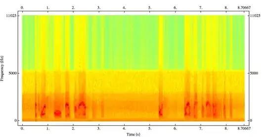
Version 9 has introduced several signal processing functions and Spectrogram is now a built-in function. You can simply do:

{data, fs} = {#[[1, 1, 1]], #[[1, 2]]} &@ExampleData[{"Sound", "Apollo11SmallStep"}];
Spectrogram[data, SampleRate -> fs, ColorFunction -> "Rainbow", 
    FrameLabel -> {"Frequency (Hz)", "Time (s)"}]

Answer 4

Mathematica can plot spectrograms using the Spectrogram function or the SpectrogramArray function, or the Fourier function -- it is very general and powerful. Here are some examples of audio spectrograms from the Wolfram demonstration site and here is a discussion on Mathematica stackexchange of the process of taking spectrograms of audio. To use mp3s you will need to convert them to .wav files, which can be done using a program like Audacity or Quicktime (or many others). If your final goal is to plot spectrograms, Audacity (or other free software) might be more appropriate. What you would gain in Mathematica is the ability to control the analysis in complete detail -- but this would not be automatic or trivial, it would take some knowledge of how the spectral functions work.