Partition data and plot each set as a different color

Question

data = { {2, 60}, {4.5, 62}, {6.5, 64}, {8, 65}, {9, 65}, {10, 
  65}, {11, 65}, {12, 67}, {13, 67}, {14, 67}, {16, 67}, {17, 
  67}, {18, 67}, {19, 65}, {20, 64}, {21, 70}, {22, 75}, {23, 
  80}, {24, 80}, {25, 82}, {26, 82}, {27, 79}, {30, 80}}

ListPlot[data, Joined -> True, 
AxesLabel -> {"T(Celcius)", "Volume Collected"}]

I want to partition the data into three pieces, and the plot produced should have the points joined with a line that corresponds to the color of the point.

One question remains: how do you want to partition your data? — Öskå, Feb 13 '14 at 19:07

ubpdqn · Answer 1 · 2014-02-16T07:38:04.283

You could use ColorFunction option . The following colors plot by paritioning of x-axis. You could choose your own function:

ListPlot[data, Joined -> True, 
 ColorFunction -> 
  Function[{x, y}, 
   Which[0 < x < 10, Red, 10 <= x < 20, Green, x >= 20, Blue]], 
 ColorFunctionScaling -> False, Mesh -> 10, MeshStyle -> None]

enter image description here

An alternative for partitioning x-values using MeshShading:

ListPlot[data, Joined -> True, Mesh -> {{10, 20}}, 
 MeshShading -> {Red, Green, Blue}]

score 4 · Answer 2 · answered Feb 13 '14 at 21:08

You haven't said how to partition the data but to automate on the basis of the length of the list you can do this:

segment = Ceiling[Length[data]/3];

ListPlot[Partition[data, segment+1, segment, 1, {}], Joined -> True, 
 AxesLabel -> {"T(Celcius)", "Volume Collected"}]

enter image description here

score 2 · Accepted Answer · answered Feb 13 '14 at 18:34

2

ListPlot[Evaluate[
  Cases[data, {a_ /; #[[1]] <= a <= #[[2]], __}] & /@ 
   Partition[{0, 10, 20, 30}, 2, 1]], Joined -> True, 
 PlotStyle -> Directive[Thick], 
 AxesLabel -> {"T(Celcius)", "Volume Collected"}]

enter image description here

answered Feb 13 '14 at 18:34

Zviovich

9,308
1
30
52

Syed · Answer 4 · 2024-02-26T17:17:40.160

data = {{2, 60}, {4.5, 62}, {6.5, 64}, {8, 65}, {9, 65}, {10, 
    65}, {11, 65}, {12, 67}, {13, 67}, {14, 67}, {16, 67}, {17, 
    67}, {18, 67}, {19, 65}, {20, 64}, {21, 70}, {22, 75}, {23, 
    80}, {24, 80}, {25, 82}, {26, 82}, {27, 79}, {30, 80}};

I will present a few variations and hopefully the readers can decide what works best for their needs.

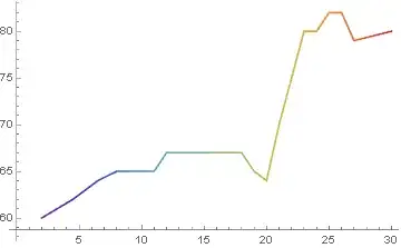
Using built in ColorData:

This is a starting point. It colors the line using the specified gradient scheme from start to finish.

ListLinePlot[data, 
 ColorFunction -> Function[{x, y}, ColorData["Rainbow"][x]]]

User defined color function with continuous change:

To color continuously in three user-defined colors from start to finish:

cf1[x_] := Blend[{Red, Blue, Green}, x];
ListLinePlot[data, ColorFunction -> (cf1[#1] &)]

User defined color function with arbitrary boundaries:

To color in discrete steps, define a ColorFunction using If. Here the cut off points are arbitrarily chosen as 8 and 15 for color boundaries.

cf2[x_] := If[x <= 8, Red, If[8 < x < 15, Blue, Darker@Green]]
ListLinePlot[data
 , ColorFunction -> (cf2[#1] &)
 , ColorFunctionScaling -> False
 , GridLines -> {{8, 15}, None}
 , GridLinesStyle -> {{Gray, Dashed}, None}
 ]

Instead of a mere color change, if data has to be partitioned and presented as such, it needs to be overlapped by one data point for it to appear continuous. e.g.

dnewOverlap = Partition[data, UpTo[9], 8]
ListLinePlot[dnewOverlap]

or

ListLinePlot[dnewOverlap, PlotStyle -> {Red, Blue, Darker@Green}]

Interested readers can add the option Mesh -> All to all plots to see the results.

Partition data and plot each set as a different color

4 Answers4

Linked