I'm trying to explore how the zeros of a certain parameterized function change as its parameter changes.
dh[n_, k_, a_] :=
dh[n, k, a] = Sum[Binomial[k, j] dh[Floor[n/(m^(k - j))], j, m + 1], {m, a, n^(1/k)}, {j, 0, k - 1}]
dh[n_, 1, a_] := Floor[n] - a + 1
dh[n_, 0, a_] := 1
bn[ z_, a_] := bn[z, a] = Product[ (z - k), {k, 0, a - 1}]/a!
dd[n_, z_] := Sum[bn[z, a] dh[n, a, 2], {a, 0, Log[2, n]}]
The function I'm exploring here is dd[n_,z_].
n is the parameter I want to vary, and is a whole number $>= 1$. The zeros are all values of z such that dd[n,z] = 0. There should be $\log_2 n$ zeros for a given n.
Now, I already know that I can see the zeros for an isolated value of n as
zeros[n_] := List @@ NRoots[ dd[n, z] == 0, z][[All, 2]]
For example, if I try zeros[30], I get {-16.1801, -1.66598 - 0.772391 I, -1.66598 + 0.772391 I, -0.0879758}
I also know that I could visualize those zeros as
RootLocusPlot[1/dd[30, z], {k, 0, 1}]
But both of these techniques only address single values of n at a time. What I really want is to see how the zeros change as n changes, particularly for different scales of ranges for n.
Does Mathematica have any tools to help me do that?
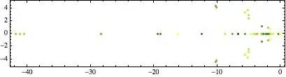
pts=Table[(Point[{Re[#], Im[#]}])& /@ zeros[n], {n, 5, 30}]and then plotting the points as inShow[Graphics[pts], Frame -> True]or some other graphics command? You could also useManipulateinstead of Table, above (with some minor modification). – Peltio Feb 27 '14 at 09:19