StreamPlot for Bifurcation Diagram

Question

When we do a StreamPlot, I want to show the bifurcation when $a = 0$ transitions to $a >0$, but do not see a better way to do this than the following.

    Animate[StreamPlot[{1,-x^4 + 5 a x^2-4 a^2}, {y,-5,5}, {x,-4,4},
                        PlotLabel -> Row[{"a = ", a}]], {a,-1,1}]

Is there a better way to show this bifurcation?

Maybe an animated gif like this Bifurcation diagrams for multiple equation systems) (this is a system and my example is not a system)?

Update

To be more clear, the original system is

$$x'(y) = -(x(y))^4 + 5a(x(y))^2 - 4a^2$$

Answer 1

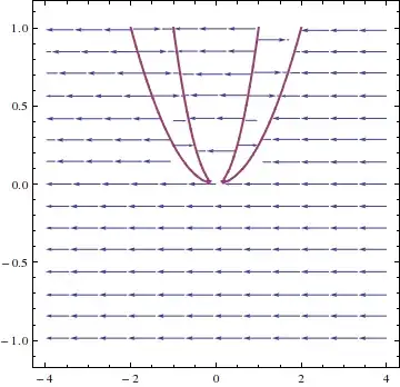
I agree with Rahul that, since you've got a single, one dimensional equation indexed by a single parameter, a bifurcation diagram is a natural way to visualize this situation. If you want an animation or dynamic image, you might highlight one particular phase line as a function of $a$. You could also display the slope field of the system right along side of the phase diagram. The result looks something like so.

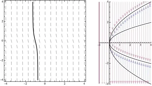
Note that I prefer to draw the solution through a simple slope field, rather than through the groovy StreamPlot because I think that's a simpler concept - particularly, for undergraduate students who I interact with a lot. I've also oriented the vertical $x$ axis in both plots in the same direction and used graphics primitives there to grab a little more control over the image.

Here's code for an interactive version of this that also includes a locator on the slope field allowing you to specify the initial condition.

Needs["DifferentialEquations`InterpolatingFunctionAnatomy`"];
Clear[slopeField, slopeFieldWithSol];
slopeField[a_?(# < 0 &)] := VectorPlot[
   {1, -x^4 + 5 a x^2 - 4 a^2}, {t, -4, 4}, {x, -4, 4},
   VectorScale -> {0.03, Automatic, None},
   VectorStyle -> {Gray, Arrowheads[0]}];
slopeField[a_?(# >= 0 &)] := Show[{
    VectorPlot[
     {1, -x^4 + 5 a x^2 - 4 a^2}, {t, -4, 4}, {x, -4, 4},
     VectorScale -> {0.03, Automatic, None},
     VectorStyle -> {Gray, Arrowheads[0]}],
    Plot[{-2 Sqrt[a], -Sqrt[a], Sqrt[a], 2 Sqrt[a]}, {t, -4, 4},
     PlotStyle -> Directive[Black, Dashed]]
    }];
slopeFieldWithSol[a_, p_] := 
  Module[{t, x, t0, x0, eq, ic, eqs, sol, xf, ifd, tRange, plot},
   {t0, x0} = p;
   eq = x'[t] == -x[t]^4 + 5 a*x[t]^2 - 4 a^2;
   ic = x[t0] == x0;
   eqs = {eq, ic};
   Quiet[sol = First[NDSolve[eqs, x, {t, -4, 4}]], NDSolve::ndsz];
   xf = x /. sol;
   ifd = InterpolatingFunctionDomain[xf];
   tRange = {t, ifd[[1, 1]], ifd[[1, 2]]};
   plot = Plot[xf[t], Evaluate[tRange], 
     PlotStyle -> {Thick, Black}, PlotRange -> {{-4, 4}, {-4, 4}}];
   Show[{slopeField[a], plot}, PlotRange -> {{-4, 4}, {-4, 4}}]
   ];     
Clear[phaseLine, phaseDiagram, phaseDiagramWithLine];
phaseLine[a_?(# < 0 &), ___] := {ColorData[1, 2], 
   Arrow[{{a, 4}, {a, -4}}]};
phaseLine[0, eps_] = phaseLine[0.0, eps_] = {ColorData[1, 2],
    Arrow[{{0, 4}, {0, eps}}], Arrow[{{0, -eps}, {0, -4}}]
    };
phaseLine[a_?(# > 0 &), eps_] := {
   Arrowheads[Medium],
   ColorData[1, 2], Arrow[{{a, 4}, {a, 2 Sqrt[a] + eps}}],
   ColorData[1, 1], 
   Arrow[{{a, Sqrt[a] + eps}, {a, 2 Sqrt[a] - eps}}],
   ColorData[1, 2], Arrow[{{a, Sqrt[a] - eps}, {a, -Sqrt[a] + eps}}],
   ColorData[1, 1], 
   Arrow[{{a, -2 Sqrt[a] + eps}, {a, -Sqrt[a] - eps}}],
   ColorData[1, 2], Arrow[{{a, -2 Sqrt[a] - eps}, {a, -4}}]
   };
phaseDiagram = ParametricPlot[{{x^2/4, x}, {x^2, x}}, {x, -4, 4},
   PlotRange -> {{-1, 4}, {-4, 4}},
   PlotStyle -> Directive[Thickness[0.007], Black],
   Epilog -> {Opacity[0.4], 
     Table[phaseLine[a, 0.1], {a, -0.7, 4, 0.2}]}];
phaseDiagramWithLine[a_] := Show[{phaseDiagram,
    Graphics[{Thick, phaseLine[a, 0.1], If[a >= 0, {PointSize[Large],
        Point[{a, #} & /@ {2 Sqrt[a], 
           Sqrt[a], -Sqrt[a], -2 Sqrt[a]}]}, {}]}]}];
Manipulate[Grid[{{
    Show[slopeFieldWithSol[a, p], ImageSize -> 300],
    Show[phaseDiagramWithLine[a], 
     ImageSize -> {Automatic, 300}]
    }}, Spacings -> 3],
 {{a, 0}, -1, 4}, {{p, {0, 1}}, {-4, -4}, {4, 4}, Locator}]

The animated gif was generated in a manner almost identical to the Manipulate. I just specified a particular p value $(-1.2,1.2)$, changed Manipulate to Table (which required me to change the a specification slightly), and Exported the result to a GIF.

pics = Table[Grid[{{
  Show[slopeFieldWithSol[a, {-1.2, 1.2}], ImageSize -> 300],
  Show[phaseDiagramWithLine[a], 
   ImageSize -> {Automatic, 300}]
  }}, Spacings -> 3],
 {a, -1, 4, 0.1}];
Export["temp.gif", pics]

Answer 2

Since you have just two variables, $x$ and $a$, you can make a 2D plot:

f[x_, a_] := -x^4 + 5 a x^2 - 4 a^2;

Show[StreamPlot[{f[x, a], 0}, {x, -4, 4}, {a, -1, 1}, StreamPoints -> Fine], 
 ContourPlot[f[x, a] == 0, {x, -4, 4}, {a, -1, 1}, ContourStyle -> ColorData[1, 2]]]

My explanatory comment below was incorrect, so I'm including a corrected version here. The parameter $a$ is on the vertical axis. For $a=1$ we have four equilibrium points. These are visible as intersections of the red curve with the slice $a=1$ parallel to the horizontal axis. Note that if you have $x'=f_a(x)=−x^4+5ax^2−4a^2$ with $a=1$, then for $|x|>2$ you have $x'<0$, for $2<|x|<1$ you have $x'>0$, and for $|x|<1$ you have $x'<0$, all of which are visible in the diagram in terms of the direction of the arrows.

Nevertheless, the version in Mark's answer is much more beautiful.