Runge-Kutta-2 on System

Question

After spending some time using the Mathematica documentation and this Mathematica.SE answer, I implemented the Runge-Kutta-2 routines.

I am hoping someone can validate what I did and tell me that it is correct (especially the Butcher Tableau I used) and the step size $h = 0.1$.

  ClassicalRungeKuttaCoefficients[4, prec_] := 
   With[{amat = {{1/2}}, bvec = {0, 1}, cvec = {1/2}}, 
    N[{amat, bvec, cvec}, prec]]

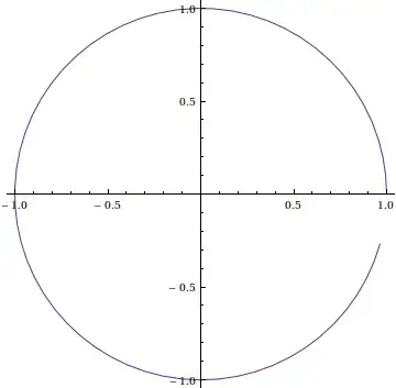
  {xf, yf} = {x, y} /. 
    First@NDSolve[{x'[t] == -y[t], y'[t] == x[t], x[0] == 1, 
     y[0] == 0}, {x, y}, {t, 0, 6}, 
     Method -> {"ExplicitRungeKutta", "DifferenceOrder" -> 4, 
    "Coefficients" -> ClassicalRungeKuttaCoefficients}, 
     StartingStepSize -> 1/10];

  xl = MapThread[Append, {xf["Grid"], xf["ValuesOnGrid"]}]

  yl = MapThread[Append, {yf["Grid"], yf["ValuesOnGrid"]}]

We can find a closed form solution to this problem as:

  s = DSolve[{x'[t] == -y[t], y'[t] == x[t], x[0] == 1, y[0] == 0}, {x, y}, t]

Lastly, is there an automated way to update and step through each variant of RK-2, RK-3, RK-4, ... without having to manually enter the Butcher values (in other words, I want to step through each variant of RK-n and compare the errors (a table of that would be great))?

There is a hint of this at Wolfram's Reference page.

Note: I am embarrassed to say that I did not totally understand ClassicalRungeKuttaCoefficients (other than the coefficients).

Answer 1

The problem with your original code is that the order argument you specified (4) is in fact not the same as the order of the midpoint method (2). Thus:

MidpointCoefficients[2, prec_] := N[{{{1/2}}, {0, 1}, {1/2}}, prec];

For comparison purposes, here's the Butcher table for Heun's method:

HeunCoefficients[2, prec_] := N[{{{1}}, {1/2, 1/2}, {1}}, prec];

We can now pass the Butcher table to NDSolve[] like so:

{xm, ym} = {x, y} /. 
  First @ NDSolve[{x'[t] == -y[t], y'[t] == x[t], x[0] == 1, y[0] == 0},
                  {x, y}, {t, 0, 6}, 
                  Method -> {"ExplicitRungeKutta", "DifferenceOrder" -> 2, 
                             "Coefficients" -> MidpointCoefficients}, 
                  StartingStepSize -> 1/10];

and check that the results are as expected:

ListLinePlot[Transpose[{xm["ValuesOnGrid"], ym["ValuesOnGrid"]}], 
             AspectRatio -> Automatic]

{Norm[xc["ValuesOnGrid"] - Cos[Range[0, 6, 1/10]], ∞], 
 Norm[yc["ValuesOnGrid"] - Sin[Range[0, 6, 1/10]], ∞]}
   {0.00813941, 0.00938408}

---

Lastly, is there an automated way to update and step through each variant of RK-2, RK-3, RK-4, ... without having to manually enter the Butcher values ... ?

In principle, one could certainly use Mathematica to solve the underlying algebraic equations satisfied by the coefficients of an $n$-th order Runge-Kutta method. But, as noted in the venerable book of Hairer/Nørsett/Wanner, the so-called order conditions very quickly become more numerous and complicated as the order is increased, so one often relies on trickery and/or approximations to generate usable higher-order coefficients. So, you could try, but you'd find it way easier to stand on the shoulders of giants.