Least Square Fitting

Question

stuck on a mathematica assignment and could really use some help.

A) Fit a function with the shape log(Y) = a0 + a1log(U) to the datapoints (log(Ui), log(Yi) with an least square fitting. Show this in a plot ...

B) Use your answer in A) to find a function Y = kU^n that fit to the datapoints (Ui, Yi)

The U datapoints is: (600000, 200000, 60000, 10000, 2500)

The Y datapoints is: (250, 60, 25, 12, 5)

I've done this:

data2 = {{Log[2500], Log[5]}, {Log[10000], Log[12]}, {Log[60000], 
   Log[25]}, {Log[200000], Log[60]}, {Log[600000], Log[250]}}

fitExample = Fit[data2, {1, x}, x]

Am I right to be using the Fit function this way? How can I use this answer in the B question?

Answer 1

You can also use LinearModelFit:

lm = LinearModelFit[data2, {1, x}, x]

You can 'normalize' output:

Normal@lm

This yields:

-3.72168 + 0.663665 x

You can look at underlying properties:

lm["Properties"]

yielding:

{"AdjustedRSquared", "AIC", "AICc", "ANOVATable", \ "ANOVATableDegreesOfFreedom", "ANOVATableEntries", \ "ANOVATableFStatistics", "ANOVATableMeanSquares", \ "ANOVATablePValues", "ANOVATableSumsOfSquares", "BasisFunctions", \ "BetaDifferences", "BestFit", "BestFitParameters", "BIC", \ "CatcherMatrix", "CoefficientOfVariation", "CookDistances", \ "CorrelationMatrix", "CovarianceMatrix", "CovarianceRatios", "Data", \ "DesignMatrix", "DurbinWatsonD", "EigenstructureTable", \ "EigenstructureTableEigenvalues", "EigenstructureTableEntries", \ "EigenstructureTableIndexes", "EigenstructureTablePartitions", \ "EstimatedVariance", "FitDifferences", "FitResiduals", "Function", \ "FVarianceRatios", "HatDiagonal", "MeanPredictionBands", \ "MeanPredictionConfidenceIntervals", \ "MeanPredictionConfidenceIntervalTable", \ "MeanPredictionConfidenceIntervalTableEntries", \ "MeanPredictionErrors", "ParameterConfidenceIntervals", \ "ParameterConfidenceIntervalTable", \ "ParameterConfidenceIntervalTableEntries", \ "ParameterConfidenceRegion", "ParameterErrors", "ParameterPValues", \ "ParameterTable", "ParameterTableEntries", "ParameterTStatistics", \ "PartialSumOfSquares", "PredictedResponse", "Properties", "Response", \ "RSquared", "SequentialSumOfSquares", "SingleDeletionVariances", \ "SinglePredictionBands", "SinglePredictionConfidenceIntervals", \ "SinglePredictionConfidenceIntervalTable", \ "SinglePredictionConfidenceIntervalTableEntries", \ "SinglePredictionErrors", "StandardizedResiduals", \ "StudentizedResiduals", "VarianceInflationFactors"}

and use for example:

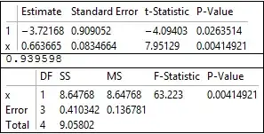
Column[{lm["ParameterTable"],
  lm["AdjustedRSquared"],
  lm["ANOVATable"]}, Frame -> All]

or 95% confidence bands for mean prediction:

p[x_] := lm["MeanPredictionBands", ConfidenceLevel -> 0.95]
Show[ListPlot[data2], Plot[Evaluate@{lm[x], p[x]}, {x, 1, 14}]]

Finally, for 'fun' you can confirm least squares result with some linear algebra:

mat = {ConstantArray[1, 5], data2[[All, 1]]};
N@Inverse[mat.Transpose@mat].mat.data2[[All, 2]]

which yields: {-3.72168, 0.663665}...as per found fit.

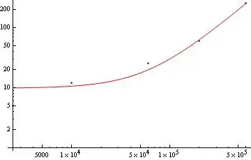
If you wish to back transform and ultimately show power relation:

tf[u_] := Exp[(Normal@lm /. x -> Log[u])]
lin = Show[ListPlot[Exp[data2]], 
  Plot[Evaluate@tf[x], {x, 2500, 600000}]]
lglg = Show[ListLogLogPlot[Exp[data2]], 
  LogLogPlot[Evaluate@tf[x], {x, 2500, 600000}]]
tf[x]

and the power relation:

0.0241932 x^0.663665

Answer 2

You may do like you started to, and then follow like in the comment of Z-Y.L. You might also go ahead directly using the FindFit function as follows. This is your initial data (without logarithms in it):

data={{2500, 5}, {10000, 12}, {60000, 25}, {200000, 60}, {600000, 250}};

here one fits it:

 ff = FindFit[data, a*x^b + c, {a, b, c}, x]

(*  {a -> 2.37535*10^-6, b -> 1.3853, c -> 9.75617}  *)

Done. Let us have a look at the data and the fit:

    Show[{
  ListLogLogPlot[data],
  LogLogPlot[a*x^b + c /. ff, {x, 2500, 600000}, PlotStyle -> Red]
  }]

It should look as follows:

Note that without the parameter c the coincidence will be still worth. Have success.