I have the following data:
test={{{15.8257, -0.0769379}, {16.1561, -0.0974535}, {16.4865,
-0.0896821}, {16.5195, -0.065402}, {16.6847, -0.0581635}, {16.8499,
-0.0702727}, {17.0151, -0.0836196}, {17.1803, -0.0888208}, {17.3455,
-0.0929545}, {17.5107, -0.105148}, {17.6759, -0.103528}, {17.8411,
-0.0836455}, {18.0063, -0.0715808}, {18.1715, -0.0650529}, {18.3366,
-0.0582498}, {18.5018, -0.0588228}, {18.667, -0.0599082}, {18.8322,
-0.0605835}, {18.9974, -0.0664554}, {19.1626, -0.0695087}, {19.3278,
-0.0696179}, {19.493, -0.0734236}, {19.6582, -0.0709082}, {19.8234,
-0.0622981}, {19.9886, -0.0673829}, {20.1538, -0.0802961}, {20.319,
-0.0798284}, {20.4842, -0.0687257}, {20.6494, -0.0717655}, {20.8146,
-0.0806611}, {20.9798, -0.085287}, {21.145, -0.0922109}, {21.3102,
-0.0944269}, {21.4754, -0.0878644}, {21.6405, -0.0880898}, {21.8057,
-0.0899869}, {21.9709, -0.078788}, {22.1361, -0.0591576}, {22.3013,
-0.044466}, {22.4665, -0.0600192}, {22.6317, -0.0748474}, {22.7969,
-0.0704493}, {22.9621, -0.0572922}, {23.1273, -0.0562575}, {23.2925,
-0.0623347}, {23.4577, -0.0634224}, {23.6229, -0.068166}, {23.7881,
-0.0829702}, {23.9533, -0.0888241}, {24.1185, -0.0735696}, {24.2837,
-0.0593534}, {24.4489, -0.0637424}, {24.6141, -0.0650974}, {24.7793,
-0.0519863}, {24.9444, -0.0404489}, {25.1096, -0.0633278}, {25.2748,
-0.0747063}, {25.44, -0.0698835}, {25.6052, -0.0770221}, {25.7704,
-0.0828237}, {25.9356, -0.0727494}, {26.1008, -0.0432394}, {26.266,
-0.0423326}, {26.4312, -0.06231}, {26.5964, -0.0736631}, {26.7616,
-0.0655702}, {26.9268, -0.0632276}, {27.092, -0.0749202}, {27.2572,
-0.0780181}, {27.4224, -0.0727166}, {27.5876, -0.0615335}, {27.7528,
-0.056091}, {27.918, -0.063779}, {28.0832, -0.0615237}, {28.2483,
-0.0506654}, {28.4135, -0.0563894}, {28.5787, -0.0836379}, {28.7439,
-0.0994342}, {28.9091, -0.0896401}, {29.0743, -0.0615194}, {29.2395,
-0.0517822}, {29.4047, -0.062227}, {29.5699, -0.0769844}, {29.7351,
-0.0813083}, {29.9003, -0.0899082}, {30.0655, -0.0893884}, {30.2307,
-0.0725808}, {30.3959, -0.050268}, {30.5611, -0.0426449}, {30.7263,
-0.0480701}, {30.8915, -0.0559944}, {31.0567, -0.0608699}, {31.2219,
-0.06694}, {31.3871, -0.0797316}, {31.5522, -0.0904721}, {31.7174,
-0.0867335}, {31.8826, -0.0808754}, {32.0478, -0.0764141}, {32.213,
-0.0672197}, {32.3782, -0.0500709}, {32.5434, -0.0431931}, {32.7086,
-0.0477298}, {32.8738, -0.0606955}, {33.039, -0.072429}, {33.2042,
-0.0820698}, {33.3694, -0.100112}, {33.5346, -0.0911248}, {33.6998,
-0.0722954}, {33.865, -0.0553945}, {34.0302, -0.0577424}, {34.1954,
   0.267945}, {34.3606, 0.580552}, {34.5258, 0.665223}, {34.6579,
   0.755472}, {34.8231, 0.759053}, {34.9883, 0.76307}, {35.1535,
   0.776505}, {35.3187,
   0.779363}, {35.4839, -1.12199}, {35.6491, -2.55552}, {35.8143,
-2.94135}, {35.9795, -3.09798}, {36.1447, -3.19286}, {36.3099,
-3.20814}, {36.4751, -3.20919}, {36.6403, -3.21143}, {36.8054,
-3.22794}, {36.9706, -3.23869}, {37.1358, -3.22691}, {37.301,
-3.22079}, {37.4662, -3.23454}, {37.6314, -3.23401}, {37.7966,
-3.21475}, {37.9618, -3.20351}, {38.127, -3.19776}, {38.2922,
-3.20082}, {38.4574, -3.20999}, {38.6226, -3.20835}, {38.7878,
-3.22132}, {38.953, -3.24514}, {39.1182, -3.23904}, {39.2834,
-3.22584}, {39.4486, -3.22737}, {39.6138, -3.21398}, {39.779,
-3.19581}, {39.9442, -3.18892}, {40.1093, -3.18855}, {40.2745,
-3.20021}, {40.4397, -3.21298}, {40.6049, -3.21224}, {40.7701,
-3.20945}, {40.9353, -3.21391}, {41.1005, -3.20505}, {41.2657,
-3.195}, {41.4309, -3.19082}, {41.5961, -3.19234}, {41.7613,
-3.19255}, {41.9265, -3.18381}, {42.0917, -3.20026}, {42.2569,
-3.2267}, {42.4221, -3.24796}, {42.5873, -3.24242}, {42.7525,
-3.23463}, {42.9177, -3.229}, {43.0829, -3.21687}, {43.2481,
-3.19914}, {43.4132, -3.17638}, {43.5784, -3.17475}, {43.7436,
-3.1944}, {43.9088, -3.22259}, {44.074, -3.23448}, {44.2392,
-3.23701}, {44.4044, -3.25577}, {44.5696, -3.25209}, {44.7348,
-3.2347}, {44.9, -3.20355}, {45.0652, -3.18403}, {45.2304, -3.1984},
{45.3956, -3.2077}, {45.5608, -3.20139}, {45.726, -3.18804},
{45.8912, -3.19259}, {46.0564, -3.22305}, {46.2216, -3.23381},
{46.3868, -3.21896}, {46.552, -3.19782}, {46.7171, -3.19925},
{46.8823, -3.21254}, {47.0475, -3.20822}, {47.2127, -3.20076},
{47.3779, -3.21503}, {47.5431, -3.23415}, {47.7083, -3.23585},
{47.8735, -3.21257}, {48.0387, -3.19277}, {48.2039, -3.21066},
{48.3691, -3.23566}, {48.5343, -3.23804}, {48.6995, -3.22519},
{48.8647, -3.22}, {49.0299, -3.22857}, {49.1951, -3.22214}, {49.3603,
-3.18748}, {49.5255, -3.17048}, {49.6907, -3.18617}, {49.8559,
-3.20105}, {50.021, -3.19556}, {50.1862, -3.19728}, {50.3514,
-3.22789}, {50.5166, -3.25828}, {50.6818, -3.252}, {50.847,
-3.22992}, {51.0122, -3.23513}, {51.1774, -3.23703}, {51.3426,
-3.19712}, {51.5078, -3.1469}, {51.673, -3.15768}, {51.8382,
-3.19598}, {52.0034, -3.22341}, {52.1686, -3.22205}, {52.3338,
-3.21716}, {52.499, -3.24412}, {52.6642, -3.25222}, {52.8294,
-3.22671}, {52.9946, -3.2061}, {53.1598, -3.21205}, {53.3249,
-3.20663}, {53.4901, -3.1892}, {53.6553, -3.18521}, {53.8205,
-3.21223}, {53.9857, -3.22453}, {54.1509, -3.21086}, {54.3161,
-3.20821}, {54.4813, -1.83753}, {54.6465, -0.497467}, {54.8117,
-0.172629}, {54.9769, -0.118185}, {55.1421, -0.0401817}, {55.3073,
-0.0390328}, {55.4725, -0.0519028}, {55.6377, -0.0341139}, {55.8029,
-0.0159919}, {55.9681, -0.0322755}, {56.1333, -0.0560436}, {56.2985,
-0.055005}, {56.4637, -0.0382538}, {56.6288, -0.0461829}, {56.794,
-0.0519669}, {56.9592, -0.0478512}, {57.1244, -0.0485063}, {57.2896,
-0.0450605}, {57.4548, -0.0328684}, {57.62, -0.0012728}, {57.7852,
   0.000699344}, {57.9504, -0.0282098}, {58.1156, -0.0528248},
{58.2808, -0.0660222}, {58.446, -0.0670143}, {58.6112, -0.0803909},
{58.7764, -0.0722626}, {58.9416, -0.056143}, {59.1068, -0.052108},
{59.272, -0.041373}, {59.4372, -0.0346966}, {59.6024, -0.0253502},
{59.7676, -0.0264026}, {59.9327, -0.0481955}, {60.0979, -0.0662766},
{60.2631, -0.068389}, {60.4283, -0.0613654}, {60.5935, -0.0516283},
{60.7587, -0.0460859}, {60.9239, -0.026215}, {61.0891, -0.0075962},
{61.2543, -0.0158598}, {61.4195, -0.0383789}, {61.5847, -0.052961},
{61.7499, -0.0406836}, {61.9151, -0.0423972}, {62.0803, -0.0769325},
{62.2455, -0.0948179}, {62.4107, -0.0665865}, {62.5759, -0.0433503},
{62.7411, -0.0465402}, {62.9063, -0.064464}, {63.0715, -0.0543498},
{63.2366, -0.0287138}, {63.4018, -0.0410531}, {63.567, -0.0596464},
{63.7322, -0.0323676}, {63.8974, -0.00447797}, {64.0626, -0.0176177},
{64.2278, -0.0278519}, {64.393, -0.0175132}, {64.5582, -0.0343388},
{64.7234, -0.0728937}, {64.8886, -0.0859438}, {65.0538, -0.0851371},
{65.219, -0.0734951}, {65.3842, -0.0496842}, {65.5494, -0.00584685},
{65.7146,
   0.0095625}, {65.8798, -0.00930119}, {66.045, -0.0250789},
{66.2102, -0.0359847}, {66.3754, -0.0667467}, {66.5405, -0.09646},
{66.7057, -0.0840331}, {66.8709, -0.0524984}, {67.0361, -0.0383522},
{67.2013, -0.0540666}, {67.3665, -0.0645649}, {67.5317, -0.0412653},
{67.6969, -0.0161336}, {67.8621, -0.037667}, {68.0273, -0.0628333},
{68.1925, -0.0356986}, {68.3577, -0.0229571}, {68.5229, -0.0403972},
{68.6881, -0.0403037}, {68.8533, -0.0353493}, {69.0185, -0.0300052},
{69.1837, -0.0497527}, {69.3489, -0.0725242}, {69.5141, -0.0655332},
{69.6793, -0.0600311}, {69.8444, -0.0536261}, {70.0096, -0.051527},
{70.1748, -0.045936}, {70.34, -0.0338074}, {70.5052, -0.0315814},
{70.6704, -0.0265081}, {70.8356, -0.0228345}, {71.0008, -0.0348291},
{71.166, -0.0534865}, {71.3312, -0.0559775}, {71.4964, -0.0523304},
{71.6616, -0.0514005}, {71.8268, -0.0403854}, {71.992, -0.0236734},
{72.1572, -0.0114473}, {72.3224, -0.0182658}, {72.4876, -0.0314441},
{72.6528, -0.0284464}, {72.818, -0.0324639}, {72.9832, -0.0492846},
{73.1483, -0.0854126}, {73.3135, -0.0898038}, {73.4787, -0.0559581},
{73.6439, -0.0413622}, {73.8091, -0.051359}, {73.9743, -0.058296},
{74.1395, -0.0417273}, {74.3047, -0.0255182}, {74.4699, -0.0485516},
{74.6351, -0.0663423}, {74.8003, -0.0699121}, {74.9655, -0.0530811},
{75.1307, -0.0473759}, {75.2959, -0.0496924}, {75.4611, -0.0424499},
{75.6263, -0.0241374}, {75.7915, -0.0436916}, {75.9567, -0.089127},
{76.1219, -0.0761635}, {76.2871, -0.0538311}, {76.4522, -0.0522625},
{76.6174, -0.0747319}, {76.7826, -0.0739987}, {76.9478, -0.0333077},
{77.113, -0.00486031}, {77.2782, -0.0153005}, {77.4434, -0.0266643},
{77.6086, -0.0274922}, {77.7738, -0.0620418}, {77.939, -0.0877488},
{78.1042, -0.0803497}, {78.2694, -0.0537084}, {78.4346, -0.0425878},
{78.5998, -0.0402573}, {78.765, -0.0197596}, {78.9302, -0.0105323},
{79.0954, -0.0277539}, {79.2606, -0.0459642}, {79.4258, -0.0416842},
{79.591, -0.0456379}, {79.7561, -0.0775024}, {79.9213, -0.0816734},
{80.0865, -0.0372224}, {80.2517, -0.0110671}, {80.4169, -0.0447514},
{80.5821, -0.073486}, {80.7473, -0.0684747}, {80.9125, -0.0510865},
{81.0777, -0.0564664}, {81.2429, -0.05117}, {81.4081, -0.0249809},
{81.5733, -0.00204501}, {81.7385, -0.0035259}, {81.9037,
-0.00623434}, {82.0689, -0.0128054}}}
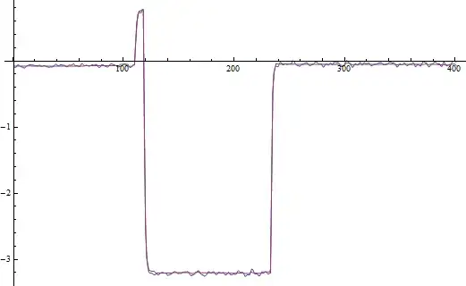
When I plot these data with Mathematica, I get the following figure:

By the way, this is a physical, non-local, spin valve signal at a given temperature.
What I need is a method to find the two switching fields (actually 4 if negative values are also considered).
At present, I doing the following:
By hand, I make two linear fits, one for the area where the signal is constant at about $-3$ mOhm, one for the area where the signal is decreasing from $0$ mOhm to $-3$ mOhm. For all temperatures, the first area is nearly the same. In the second area, where is this strong decrease of the signal, I have to fit the line by hand. For this example it would be:
{{35.3187, 0.779363}, {35.4839, -1.12199}, {35.6491, -2.55552},
 {35.8143, -2.94135}, {35.9795, -3.09798}}
From these two lines, I get the intersection point which is what I am interessted in.
This method takes me about 10 min for each intersection point because I have to do it by hand, which is OK for one data set. For the 240 data sets that I have this would take a relativly long time, so I'm looking for a way to automate it.
The final result looks like this :
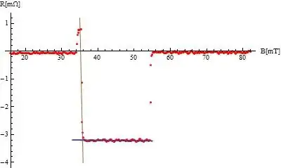
What I find especially difficult is getting Mathematica to find the correct values for the second line, because I usually have just 3 or 4 measured points for such lines.
I hope someone will respond with some nice ideas how this can be done automatically.