Orthogonal Graph layout

Question

Is it possible for Mathematica to layout a graph so that the connections lie on a grid? Furthermore, for graphs with multiple edges per vertex, is it possible to specify the location on the vertex for each connection? The context of this question is to use Mathematica's graph functionality to represent / visualize networks of circuit components. Each component has some number of input and output ports and I would like to be able to generate a network layout based on a connectivity map (netlist). I've been using GraphPlot and LayeredGraphPlot and have looked through quite a few different options but none that quite address these issues.

===== EDIT (by @VitaliyKaurov): ====

Reading @Szabolcs and @gsarma comments I am posting the image they to refer and which is approximately what is needed.

enter image description here

Can the edges turn 90 degrees, or are they always straight (i.e. the graph is very special)? @R.M I think he means that he already has a graph, and needs to lay it out so that all edges run along a square grid. — Szabolcs, May 11 '12 at 08:12
@Szabolcs Then he should create a custom grid using Table (or other means) and set it via VertexCoordinates. I do that in my boggle answer (see last part). — rm -rf, May 11 '12 at 08:18
@R.M But it might not be a full grid. Maybe it's a graph with only 20 vertices, and it's being laid out on a 10 by 10 grid. Maybe the edge lengths can be any multiples of the cell size of the grid. "Fitting" the graph onto the grid (i.e. calculating the correct VertexCoordinates) becomes not so trivial in this case. This is how I understand the question, but I agree it needs clarification. — Szabolcs, May 11 '12 at 08:29
@wilbert van meerwijk: VertexCoordinateRules allows one to specify the coordinates of the vertices, and I'm assuming this is what I will have to use in order to write my own automated layout routine, but I was curious if any of the built-in embeddings would constrain connections to lie on a lattice. — systematic, May 11 '12 at 08:35
@Szabolcs: Yes, there can be corners between the vertices. In effect, I would like a graph representation of a system model, for example, that one might design in MathModelica. Perhaps future versions of MathModelica / Graphs and Networks / Control Systems will include something along these lines. In particular, it seems that the ability to specify "ports" for vertices would be necessary for the block diagrams in the Control Systems documentation to be actual symbolic expressions. At present, it seems that they are simply included graphics. — systematic, May 11 '12 at 08:35
@gsarma To clarify what you need: please open this page (needs Flash) first, then in the web application click Help -> Example Graphs -> Computer Network. Then click Layout -> Orthogonal. Are you asking for doing the same in Mathematica was Layout -> Orthogonal does there? — Szabolcs, May 11 '12 at 08:40

Vitaliy Kaurov · Accepted Answer · 2014-04-23T18:03:03.280

=== UPDATE ===

Functionality and concept are updated and discussed here:

Orthogonal aka rectangular edge layout for Graph

=== OLDER ===

The main problem here I think is laying out edges along orthogonal lines. This can be addressed with splines. First define function that triples every element in the list to make a spline to pass sharply through the points.

mlls[l_] := Flatten[Transpose[Table[l, {i, 3}]], 1];

In the function below I'll define a special EdgeRenderingFunction, a trick learned from @Yu-SungChang . Using LayeredGraphPlot:

OrthoLayer[x_] := LayeredGraphPlot[x, VertexLabeling -> True,
  PlotStyle -> Directive[Arrowheads[{{.02, .8}}], GrayLevel[.3]],

  EdgeRenderingFunction -> (Arrow@
      BezierCurve[
       mlls[{First[#1], {(1 First[#1][[1]] + 2 Last[#1][[1]])/3, 
          First[#1][[2]]}, {(1 First[#1][[1]] + 2 Last[#1][[1]])/3, 
          Last[#1][[2]]}, Last[#1]}]] &)]

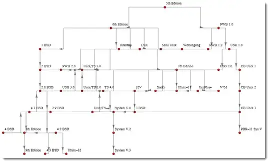
Now I will use data from HERE and test the function

OrthoLayer[g]

enter image description here

Or similarly using Graph function:

OrthoLayer[x_] := Graph[x,
   GraphLayout -> "LayeredDrawing",
  VertexLabels -> "Name", VertexSize -> .1, VertexStyle -> Red,
  EdgeStyle -> Directive[Arrowheads[{{.015, .8}}], GrayLevel[.3]],
  EdgeShapeFunction -> (Arrow@
      BezierCurve[
       mlls[{First[#1], {(1 First[#1][[1]] + 2 Last[#1][[1]])/3, 
          First[#1][[2]]}, {(1 First[#1][[1]] + 2 Last[#1][[1]])/3, 
          Last[#1][[2]]}, Last[#1]}]] &), 
  PlotRange -> {{-.1, 4.4}, {-.1, 2.5}}]

OrthoLayer[g]

enter image description here

Using splines allows us to take advantage of various GraphLayout settings and still keep orthogonal edges.

g = {"John" -> "plants", "lion" -> "John", "tiger" -> "John", 
   "tiger" -> "deer", "lion" -> "deer", "deer" -> "plants", 
   "mosquito" -> "lion", "frog" -> "mosquito", "mosquito" -> "tiger", 
   "John" -> "cow", "cow" -> "plants", "mosquito" -> "deer", 
   "mosquito" -> "John", "snake" -> "frog", "vulture" -> "snake"};

OrthoLayer[x_, st_] := 
 Graph[x, GraphLayout -> st, VertexLabels -> "Name", VertexSize -> .3,
   VertexStyle -> Red, 
  EdgeStyle -> Directive[Arrowheads[{{.015, .8}}], GrayLevel[.3]], 
  EdgeShapeFunction -> (Arrow@
      BezierCurve[
       mlls[{First[#1], {(1 First[#1][[1]] + 2 Last[#1][[1]])/3, 
          First[#1][[2]]}, {(1 First[#1][[1]] + 2 Last[#1][[1]])/3, 
          Last[#1][[2]]}, Last[#1]}]] &), PlotRange -> All, 
  PlotRangePadding -> .2]

OrthoLayer[g, #] & /@ {"CircularEmbedding", "LayeredDrawing", 
  "RandomEmbedding", "SpiralEmbedding", "SpringElectricalEmbedding", 
  "SpringEmbedding"}

enter image description here

Not perfect, but a start. Many things can be adjusted to customize specific data.

Thank you Vitaliy- this was extremely helpful. – systematic Jul 12 '12 at 18:38 — systematic, Jul 12 '12 at 18:38

Verbeia · Answer 2 · 2012-06-22T21:32:42.790

Consider a sample graph.

g = RandomGraph[BernoulliGraphDistribution[10, 0.5]]

enter image description here

We can get the actual vertex list like this:

PropertyValue[{g, #}, VertexCoordinates] & /@ VertexList[g]
(*  {{2.74373, 0.537705}, {1.34615, 1.02584}, {1.82543, 1.22826}, {0., 
   0.531856}, {0.755493, 0.678809}, {1.4028, 2.11914}, {0.991734, 
   0.}, {1.74247, 0.190579}, {0.84817, 1.39096}, {1.94835, 0.6529}} *)

We can shift those vertices onto a grid by rounding the coordinates in a suitable way (note Round is Listable):

ongrid = Round[
   PropertyValue[{g, #}, VertexCoordinates] & /@ VertexList[g], 1/2]

We can then apply these new coordinate rules to the original graph through a slightly convoluted use of SetProperty.

g2 = Fold[SetProperty[{#1, #2[[1]]}, VertexCoordinates -> #2[[2]]] &, 
   g, Transpose[{VertexList[g], ongrid}] ]

enter image description here

This can all be bound up in a custom function like so:

Clear[LayoutOnGrid]

LayoutOnGrid[g_Graph, d_?NumericQ] :=
 Module[{v = VertexList[g], grid}, 
  grid = Round[
    PropertyValue[{g, #}, VertexCoordinates] & /@ v, d];
  Fold[SetProperty[{#1, #2[[1]]}, VertexCoordinates -> #2[[2]]] &, g, 
   Transpose[{v, grid}] ]]

Note that you might need to tweak how to round the coordinate locations to get a nice look. Rounding to 1 tends to put lots of vertices on top of each other.

LayoutOnGrid[RandomGraph[BernoulliGraphDistribution[20, 0.5]], 1/2]

enter image description here

Thank you Verbeia- this was good to know as well. – systematic Jul 12 '12 at 18:37 — systematic, Jul 12 '12 at 18:37

Orthogonal Graph layout

2 Answers2

Linked