Plotting an implicit polar equation

Question

Mathematica can use ContourPlot to draw implicit Cartesian equations, but doesn't seem to have a similar function to plot an implicit polar equation, for example

$\theta ^2=\left(\frac{3 \pi }{4}\right)^2 \cos (r)$

What's the best way to do this?

Well, it's a good question and I see solutions people are coming up with are different. Always interesting to see and compare, no harm in it. — Vitaliy Kaurov, Jan 23 '12 at 20:39
@David can I ask why you removed the "storytelling paragraph"? I only wanted to let people know that I planned to answer myself, and would have deleted it myself later. — one-more-minute, Jan 23 '12 at 20:56
We don't want to discourage people from answering questions. Even if you have one solution, there might be others that are enlightening for yourself or others. — Brett Champion, Jan 23 '12 at 21:01
Makes sense, I just didn't want to make others spend their time repeating a solution I already have written out. Nevermind, as you said, all contributions are helpful. — one-more-minute, Jan 23 '12 at 21:09

score 26 · Accepted Answer · answered Jan 23 '12 at 20:35

26

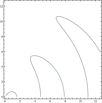
Since ContourPlot[] returns a GraphicsComplex, you could also replace the point list of the plot with g @@@ pointlist where g is the coordinate transformation. For example

f[r_, th_] := th^2 - (3 Pi/4)^2 Cos[r]
g[r_, th_] := {r Cos[th], r Sin[th]} 

pl = ContourPlot[f[r, th] == 0, {r, 0, 8 Pi}, {th, 0, 2 Pi}, PlotPoints -> 30];
pl[[1, 1]] = g @@@ pl[[1, 1]];

Show[pl, PlotRange -> All]

which produces

Mathematica graphics

The advantage of this method is that it also works for coordinate transformations for which the inverse transformation is hard to find.

answered Jan 23 '12 at 20:35

Heike

35,858
3
108
157

1

cheeky, cheeky... +1 – acl Jan 23 '12 at 20:43
4

Very interesting point, applying the coordinate transformation to the finished plot. However, I think this might fail for high frequency functions/coordinate systems etc., since after plotting things like the step distance between points are already set. – David Jan 23 '12 at 20:46
This is basically what I ended up doing, I turned it into a self-contained function so I'll post it up later. +1 for reading my mind. @David I did find that quality was reduced but bumping up MaxRecursions helps without slowing things down too much. – one-more-minute Jan 23 '12 at 20:49
1

I would include AspectRatio -> Automatic in Show so that this "looks nice." – Mr.Wizard Jan 24 '12 at 14:20
It doesn't work in version 13. It should be pl[[1, 1, 1]] = g @@@ pl[[1, 1, 1]]; – yode Jan 03 '22 at 19:21

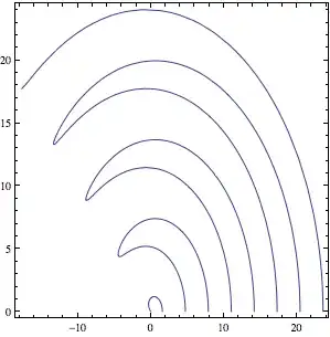
score 13 · Answer 2 · edited Mar 09 '19 at 05:44

13

Does this

ContourPlot[
 Evaluate@With[
   {r = Sqrt[x^2 + y^2],
    θ = ArcTan[x, y]},
   θ^2 - Cos[r] == 0
   ],
 {x, 0.1, 4 Pi}, {y, 0, 4 Pi}
 ]

work?

Plot:

Mathematica graphics

edited Mar 09 '19 at 05:44

Mr.Wizard

271,378
34
587
1,371

answered Jan 23 '12 at 20:30

acl

19,834
3
66
91

This is a great method, unfortunately it's not as useful if you want to specify the plotting range in polar, rather than cartesian, coordinates. +1 for your ContourPlot substitution, this is something I tried originally but couldn't get to work. – one-more-minute Jan 23 '12 at 21:17
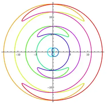
@myk thanks, Heike's is definitely cleverer and also more useful if you can't invert the transformation easily – acl Jan 23 '12 at 21:20

score 10 · Answer 3 · answered Jan 24 '12 at 03:55

If you allow negative radii, there's another entire half of the solution:

PolarPlot[
   Evaluate[Flatten[
      Table[{-ArcCos[(16 t^2)/(9 Pi^2)], ArcCos[(16 t^2)/(9 Pi^2)]} + k 2 Pi, 
            {k, -2, 2}]
      ]], 
   {t, -Pi, Pi}, 
   PlotStyle -> Table[Directive[Thick, Hue[i/10]], {i, 10}]
   ]

enter image description here

score 9 · Answer 4 · edited Jan 23 '12 at 21:49

9

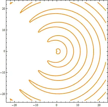
You can do something like this:

ContourPlot[ArcTan[x,y]^2 == (3 Pi/4)^2 Cos[Sqrt[x^2 + y^2]], 
{x, -23, 23}, {y, -23, 23}, ContourStyle -> Directive[Thick, Orange]]

enter image description here

edited Jan 23 '12 at 21:49

Brett Champion

20,779
2
64
121

answered Jan 23 '12 at 20:31

Vitaliy Kaurov

73,078
9
204
355

I think you're still missing a square on the 3Pi/4. – Brett Champion Jan 23 '12 at 21:21
@BrettChampion Yes, thanks, have to get my math straight ;-) – Vitaliy Kaurov Jan 24 '12 at 02:15

score 8 · Answer 5 · edited Jun 16 '20 at 09:23

All the other three solutions use ContourPlot. Here's a solution using PolarPlot.

PolarPlot[{ArcCos[#2^2/(3 π/4)^2] + 2 π #1, 
    -ArcCos[#2^2/(3 π/4)^2] + 2 π (#1 + 1)} & @@ QuotientRemainder[Abs@ θ, 2 π], 
    {θ, -7 π, 8 π}, PlotStyle -> {Thick, Darker@Green}]

enter image description here

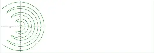
This makes use of the fact that the solution to $\theta^2=\displaystyle\left(\frac{3\pi}{4}\right)^2\cos(r)$ is

$$r=\pm\arccos\left(\frac{16\theta^2}{9\pi^2}\right)+2\pi n,\ n\in\mathbb{Z}$$

Plotting an implicit polar equation

5 Answers5

Linked

Related