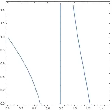
2

Condsider

function = Tan[1 x] + Tan[2 x]
Plot[function, {x, 0, 1.5}]

enter image description here

It has a strong discontinuity around 0.8.

The problem is , if I want to find function==0, Mathematica will not only find the real root x~1.1 , but also a artifact root x~0.8 Because I think Mathematica created a line around the discontinuity. A single point the has its y value of all values, which I call "a point that is every point".

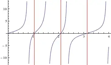
To make this obvious, let me make a Contour Plot:

ContourPlot[function + 2*y == 0, {x, 0, 1.5}, {y, 0, 1.5}, PlotPoints -> 100]

enter image description here

We know that only curved line represents real roots. The constant line is the artifact. In fact, if you plot contour for function + 2*y == 1 or function + 2*y == 2, this artifact line remains. Of course, since it is a point that is every point:

ContourPlot[function + 2*y == 1, {x, 0, 1.5}, {y, 0, 1.5}, PlotPoints -> 100]
ContourPlot[function + 2*y == 2, {x, 0, 1.5}, {y, 0, 1.5}, PlotPoints -> 100]

enter image description here enter image description here

So, how to solve the problem in Contour Plot if function to plot has a strong discontinuity that Mathematica tries wrongly (hard) to connect.

m_goldberg
  • 107,779
  • 16
  • 103
  • 257
bboczeng
  • 449
  • 5
  • 9

2 Answers2

2

If want solution without artefact, then use NSolve. And use Exclusions to avoid the divergence line

f[x_]:=Tan[1 x]+Tan[2 x]
sol=x/.NSolve[f[x]==0 && 0<x<4, x] (*finds all solutions for 0<x<4*)
Plot[f[x], {x, 0, 4}, GridLines -> {sol, {0}}, GridLinesStyle -> Red,  Exclusions -> 1/f[x] == 0]

The result you get is {1.0472,2.0944,3.14159}, free from a point that is every point.

enter image description here

You can omit the line that corresponds a divergence from ContourPlot also using Exclusions.

g[x_, y_] = f[x] + 2*y
ContourPlot[g[x, y] == 1, {x, 0, 1.5}, {y, 0, 1.5}, PlotPoints -> 100,  Exclusions -> 1/g[x, y] == 0]

enter image description here

Sumit
  • 15,912
  • 2
  • 31
  • 73
1

At least with V10 you get the desired results as follows (I can't show the images because my trial version doesn't allow that):

function = Tan[1 x] + Tan[2 x];

Plot[function, {x, 0, 1.5}, Exclusions -> Cot[2 x] == 0]

ContourPlot[function + 2*y == 1, {x, 0, 1.5}, {y, 0, 1.5},
 PlotPoints -> 100,
 Exclusions :> Cot[2 x] == 0]

sol = Table[FindRoot[function == 0, {x, i}], {i, 0, 1.5, 0.1}] /. 
 Rule[_, a_] :> Round[a, 0.0001] // Flatten // Chop // Union

Mathematica graphics Mathematica graphics

{0., 1.0472}

New in V10:

NumberLinePlot[function == 0,
 {x, 0, 1.5},
 AspectRatio -> 0.5,
 Frame -> True,
 FrameTicks -> {{None, None}, {sol, None}},
 GridLines -> {sol, None},
 GridLinesStyle -> Dashed,
 PlotTheme -> "Detailed"]

Mathematica graphics

PS - You can find the poles with

Reduce[function > 10^6, x] /. C[1] -> 0 // N // Flatten // Sort

-2.35619 < x < -2.35619 || -1.5708 < x < -1.5708 || -0.785399 < x < -0.785398 || 0.785398 < x < 0.785398 || 1.5708 < x < 1.5708 || 2.35619 < x < 2.35619

eldo
  • 67,911
  • 5
  • 60
  • 168