How do I plot a function over a subset of the displayed interval?

Question

I want to plot f1[x] over 0 < x < L/2 and f2[x] over L/2 < x < L (i.e. so that f1[x] isn't displayed overL/2 < x < L, etc.). How do I do this?

Answer 1

As b.gatessucks commented, use Piecewise. For example:

f1[x_] := Sin[x]
f2[x_] := Cos[x]
L = 7;
pw = Piecewise[{{f1@#, 0 < # < L/2}, {f2@#, L/2 < # < L}}, Indeterminate] &;
Plot[pw[x], {x, 0, L}]

Generally you should not use capital letters for variable names (L) but I kept your notation in this case.

Answer 2

We needn't use Piecewise, alternatively one can use Condition (/;) and/or ConditionalExpression (new in version 8).

f1[x_] := Sin[x]
f2[x_] := Cos[x]

Here are respective definitions :

f[x_] /; 0 <= x <= Pi := f1[x]
f[x_] /; Pi < x <= 2 Pi := f2[x]

or a sligtly different way :

ff[x_] /; x <= L/2 := f1[x]
ff[x_] /; L/2 < x  := f2[x]

we can do a similar construction in a more flexible way assuming e.g. dependence of the function on the parameter L :

g[x_, L_] /; 0 <= x <= L    := ConditionalExpression[f1[x], 0 <= x <= L]
g[x_, L_] /; L <  x <= 2 Pi := ConditionalExpression[f2[x], L < x <= 2 Pi]

to plot these functions we can make use of e.g. Exclusions option, let's demonstrate how it works :

GraphicsRow[{ Plot[f[x], {x, 0, 2 Pi}, Exclusions -> {x == Pi}],
              Plot[f[x], {x, 0, 2 Pi}] }]

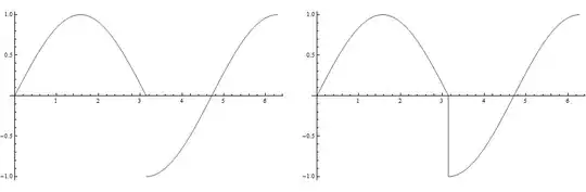
In case of ff function we can use RegionFunction option, to plot an appropriately restricted range, e.g.

L = 2 Pi;
GraphicsRow[{ Plot[ ff[x], {x, 0, L}, Exclusions -> {x == Pi}, PlotStyle -> Thick], 
              Plot[ ff[x], {x, -Pi/2, 5/2 Pi}, Exclusions -> {x == Pi}, 
                    PlotStyle -> Thick, RegionFunction -> Function[{x, y}, L > x > 0]] }]

We show here something more customized :

Animate[ Plot[ g[x, L], {x, 0, 2 Pi}, PlotRange -> {{0, 2 Pi}, {-1.05, 1.05}},
              Exclusions -> {x == L}, PlotStyle -> Thickness[0.01],
              ColorFunction -> "DeepSeaColors", ImageSize -> {500, 500}], 
         {L, 0, 2 Pi}]

Answer 3

Or without the use of piecewise:

gg1 = Plot[Cos[x], {x, \[Pi]/2 + $MachineEpsilon, \[Pi]}];
gg2 = Plot[Sin[x], {x, 0, \[Pi]/2}];

Show[gg2, gg1, PlotRange -> {{0, \[Pi]}, {-1, 1}}]

Here is a more integrated version with it bundled up into a function which takes a list of functions to plot and an arbitrary number of ranges:

Clear[DisjointRangePlot2D];
DisjointRangePlot2D[fs_List, xRanges_List] := 
 Module[{x}, 
  Show[MapThread[
    Plot[#1[x], Evaluate@Flatten@{x, #2}] &, {fs, xRanges}], 
   PlotRange -> {{Min@First@(xRanges\[Transpose]), 
      Max@Last@(xRanges\[Transpose])}, Automatic}]]
DisjointRangePlot2D[f_, xRanges_List] := 
 DisjointRangePlot2D[Table[f, {Length@xRanges}], xRanges]

A selected plot with a single function:

DisjointRangePlot2D[Sin, {{0, \[Pi]}, {2 \[Pi], 4 \[Pi]}, {7 \[Pi], 10 \[Pi]}}]

A plot with multiple functions and ranges:

DisjointRangePlot2D[{Sin, Cos, Cos}, {{0, \[Pi]}, {2 \[Pi], 4 \[Pi]}, {7\[Pi], 10 \[Pi]}}]

I did play with passing opts:OtpionsPattern[] to Plot or Show to give more control over the final output, but I didn't succeed in making that work.

Answer 4

Piecewise would work but displays a spurious line at 0 vertical coordinate:

f[x_] := Sin[x];
Plot[Piecewise[{{f[x], x < 2 Pi}}], {x, 0, 4 Pi}]

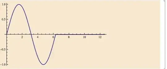
(note the horizontal line for $x>2\pi$).

One can avoid this by simply displaying a bigger range than has been plotted, as follows:

Show[
 Plot[f[x], {x, 0, 2 Pi}],
 PlotRange -> {{0, 4 Pi}, {-1, 1}}
 ]

There is now nothing at $x>2\pi$.