2D Fourier transform of a few (4) disjoint discs on a plane

Question

I'd really appreciate some advice.

Short Version

I'm trying to calculate the following $$ \psi(X,Y,z=d)=\underset{aperature}{\iint}\psi(x,y,z=0)e^{-i\frac{k}{d}\left(xX+yY\right)}dxdy\\\psi(x,y,z=0)={\sum}\left[\delta\left(x-x_{i}\right)\delta\left(y-y_{i}\right)e^{ih_{i}k}\right]\otimes circ(\sqrt{x_{i}^{2}+y_{i}^{2}}) $$

Long version

For an optics project, i'm trying to use Mathematica to perform a 2D Fourier Transform of 4 discs where each disc has a complex exponent representing its constant, relative phase (discs = functions who are 1*e^(i*phase) if inside the disc and 0 else). Disc centers are at different points in the plane, and the discs are disjoint.

I'm very new to Mathematica and not finding a better way around, have been trying to use NIntegrate to numerically asses and plot (using Plot3D) the FT of the discs, having expressed them in Cartesian coordinates.

Besides being a nightmare to write, I can't get the code to finish running since the integrals are very oscillatory and Mathematica keep sending me these notifications:

"Numerical integration converging too slowly; suspect one of the \ following: singularity, value of the integration is 0, highly \ oscillatory integrand, or WorkingPrecision too small."

I know there are no singularities since when I calculate each integral separately from the rest with smaller phase (so it won't oscillate allot) I do manage to get a correct 3D plot. However, when all of the integrals are calculated together, the calculation takes forever (I quit the kernel after about half an hour of running).

It'd really help if someone could advise me on how to write this code or suggest a simpler way to do this (there must be one). As I mentioned, I'm very new to Mathematica and so thorough explanations would help allot and be very much appreciated.

I'm attaching my code so far for reference.

My code:

\*discs radius*\
ρ = 1; 
\*constants that determine phase*\
k = (2 π)/(0.5 10^-6); 
d = 2; 
Subscript[h, 1] = 0.001;
Subscript[h, 2] = 0.002;
Subscript[h, 3] = 0.003;
Subscript[x, 1] = 0;
Subscript[y, 1] = 0.03;
Subscript[x, 2] = 0.035;
Subscript[y, 2] = 0.01;
Subscript[x, 3] = 0.025;
Subscript[y, 3] = 0.02;

Plot3D[(Abs[ -((I k )/d) π ρ^2 ((
  2 BesselJ[1, k/d  ρ Sqrt[u^2 + v^2]])/(
  k/d  ρ Sqrt[u^2 + v^2])) - (2 I)/
 v  ( E^(I k/d (Subscript[h, 1] - v Subscript[y, 1])) (  
     NIntegrate[
       E^(-I  u x k/
         d) (E^(-I v k/
           d  (ρ^2 - ( x - Subscript[x, 1])^2)^0.5) - 1), {x,
         Subscript[x, 1], Subscript[x, 1] + ρ}, 
       MaxRecursion -> 5000] + 
      NIntegrate[
       E^(-I  u x k/
         d) (E^(-I v k/
           d  (ρ^2 - ( x - Subscript[x, 1])^2)^0.5) - 1), {x,
         Subscript[x, 1] - ρ, Subscript[x, 1]}, 
       MaxRecursion -> 5000] + 
      NIntegrate[
       E^(-I  u x k/
         d) (1 - E^(
          I v k/d (ρ^2 - ( x - Subscript[x, 1])^2)^0.5)), {x,
         Subscript[x, 1] -ρ, Subscript[x, 1]}, 
       MaxRecursion -> 5000] + 
      NIntegrate[
       E^(-I  u x k/
         d) (1 - E^(
          I v k/d (ρ^2 - ( x - Subscript[x, 1])^2)^0.5)), {x,
         Subscript[x, 1], Subscript[x, 1] + ρ}, 
       MaxRecursion -> 5000]) + 
   E^(I k/d (Subscript[h, 2] - v Subscript[y, 2])) (  
     NIntegrate[
       E^(-I  u x k/
         d) (E^(-I v k/
           d  (ρ^2 - ( x - Subscript[x, 2])^2)^0.5) - 1), {x,
         Subscript[x, 2], Subscript[x, 2] + ρ}, 
       MaxRecursion -> 5000] + 
      NIntegrate[
       E^(-I  u x k/
         d) (E^(-I v k/
           d  (ρ^2 - ( x - Subscript[x, 2])^2)^0.5) - 1), {x,
         Subscript[x, 2] - ρ, Subscript[x, 2]}, 
       MaxRecursion -> 5000] + 
      NIntegrate[
       E^(-I  u x k/
         d) (1 - E^(
          I v k/d (ρ^2 - ( x - Subscript[x, 2])^2)^0.5)), {x,
         Subscript[x, 2] -ρ, Subscript[x, 2]}, 
       MaxRecursion -> 5000] + 
      NIntegrate[
       E^(-I  u x k/
         d) (1 - E^(
          I v k/d (ρ^2 - ( x - Subscript[x, 2])^2)^0.5)), {x,
         Subscript[x, 2], Subscript[x, 2] + ρ}, 
       MaxRecursion -> 5000]) + 
   E^(I k/d (Subscript[h, 3] - v Subscript[y, 3])) (  
     NIntegrate[
       E^(-I  u x k/
         d) (E^(-I v k/
           d  (ρ^2 - ( x - Subscript[x, 3])^2)^0.5) - 1), {x,
         Subscript[x, 3], Subscript[x, 3] + ρ}, 
       MaxRecursion -> 5000] + 
      NIntegrate[
       E^(-I  u x k/
         d) (E^(-I v k/
           d  (ρ^2 - ( x - Subscript[x, 3])^2)^0.5) - 1), {x,
         Subscript[x, 3] - ρ, Subscript[x, 3]}, 
       MaxRecursion -> 5000] + 
      NIntegrate[
       E^(-I  u x k/
         d) (1 - E^(
          I v k/d (ρ^2 - ( x - Subscript[x, 3])^2)^0.5)), {x,
         Subscript[x, 3] -ρ, Subscript[x, 3]}, 
       MaxRecursion -> 5000] + 
      NIntegrate[
       E^(-I  u x k/
         d) (1 - E^(
          I v k/d (ρ^2 - ( x - Subscript[x, 3])^2)^0.5)), {x,
         Subscript[x, 3], Subscript[x, 3] + ρ}, 
       MaxRecursion -> 5000]))])^2, {u, -0.001, 
  0.001}, {v, -0.001, 0.001}]

Answer 1

Here's a qualitative way to do the computation using FFTs. First, make some data (in this, the disks all have phase 1, but that can be easily fixed):

w1 = 600;
w2 = 800;
dat = Sum[
   RotateRight[
    DiskMatrix[
     RandomInteger[{1, 150}], {w1, 
      w2}], {RandomInteger[{-1000, 1000}], 
     RandomInteger[{-1000, 1000}]}], {k, 6}];

Here's a plot of the data:

Image[0.5 dat, Magnification -> 1]

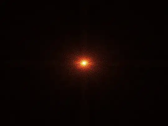
Then you can plot the frequency domain picture like this:

<< Developer`
Image[RotateRight[
   Abs[Fourier[dat]], {w1/2, w2/2}]\[TensorProduct]ToPackedArray[{1.0,
     0.3, 0.1}], Magnification -> 1]