How to define multiple functions using a for command

Question

Let's say I want to plot 10 graphs of those following functions. Since they are recursive functions, I cant make a table with 10 different initial conditions because Mathematica stores each value individually.

Then, I could define p1...p10 and θ1...θ10 manually and just make a Show[graph1...graph10]

However, how can I define the functions in an fast way doing something like that:

For[i = 1, i < 10, i++;
 θi[j_] := θi[j] = θi[j - 1] + β*pi[j - 1];
 pi[j_] := pi[j] = pi[j - 1] - α*Sin[θi[j - 1] + β*pi[j - 1]];
 θi[0] = Pi/4+i/10; 
 pi[0] = 0.8-i/10;
 graphi = ListPlot[Table[{θi[j], pi[j]}, {j, 0, 100}], AxesLabel -> {"θ(j)", "p(j)"}]]

so I can join the functions plot in a Show later?

Answer 1

You ought to set up functions that are indexed by i, not just looped through and reusing the same names. Why use θi when you could use θ[i]?

α=0.2;β=0.1;
For[i = 1, i < 10, i++,
 θ[i][j_] := θ[i][j] = θ[i][j - 1] + β*p[i][j - 1];
 p[i][j_] := p[i][j] = p[i][j - 1] - α*Sin[θ[i][j - 1] + β*p[i][j - 1]];
 θ[i][0] = Pi/4+i/10; 
 p[i][0] = 0.8-i/10;
 graph[i] = ListPlot[
  Table[{θ[i][j], p[i][j]}, {j, 0, 100}],
  PlotStyle -> RGBColor[{1 - i/10, i/15, i/10}]
 ]
]

All I did was make every instance of i in a variable name into a parameter [i]. Also watch out! You have a semicolon after i++ when you should have a comma. And the important plot option, color, is here, while the axes labels are relegated to the Show command (below).

If you want these to vary with α and β, I suggest you also include them as arguments, e.g. θ[i][α_,β_,j_] or similar.

I don't want to change your code too much, so I mostly just replaced i with [i]. However, you could also avoid the use of a loop entirely (if you're really interested, comment and I can follow up) because now you are just defining ten separate functions.

Anyway, after that, all you need is:

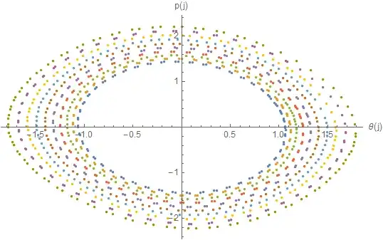
Show[Table[graph[i], {i, 1, 9}],
 AxesLabel -> {"θ(j)", "p(j)"}, PlotRange -> All
]

I added the color options so that you can see which is which. With these parameter values they look like ellipses. I also started by setting values for your parameters. If they are not numerical, you can't plot them, so I went ahead and assumed you have them. Note that in addition to not giving you an actual graph, if α and β are symbolic, the recursion becomes a symbolic nightmare computing a table of 100 recursions of some symbolic expression.

Answer 2

You can use Table if you Clear within the loop:

α = 0.2; β = 0.1;

Table[
  Clear[θi, pi];
  θi[j_] := θi[j] = θi[j - 1] + β*pi[j - 1];
  pi[j_] := pi[j] = pi[j - 1] - α*Sin[θi[j - 1] + β*pi[j - 1]];
  θi[0] = Pi/4 + i/10;
  pi[0] = 0.8 - i/10;
  Table[{θi[j], pi[j]}, {j, 0, 100}],
  {i, 10}
] // ListPlot[#, AxesLabel -> {"θ(j)", "p(j)"}] &

Using NestList makes all this simpler however:

α = 0.2; β = 0.1;

Table[
  NestList[
    {# + β #2, #2 - α*Sin[# + β #2]} & @@ # &,
    {Pi/4 + i/10, 0.8 - i/10},
    100
  ],
  {i, 10}
] // ListPlot[#, AxesLabel -> {"θ(j)", "p(j)"}] &

Although not general you can even utilize the listability (vector computation) of all constituent operations in your functions to turn the problem inside out:

ListPlot[
  NestList[{# + β #2, #2 - α*Sin[# + β #2]} & @@ # &,
    {Pi/4 + #/10, 0.8 - #/10} & @ Range @ 10, 100] ~Transpose~ {2, 3, 1},
  AxesLabel -> {"θ(j)", "p(j)"}
]