Mapping StreamPlot onto spherical surfaces

Question

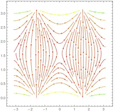
Suppose I have some vector field equations $(f(\theta,\phi), g(\theta,\phi))$. The StreamPlot can be created easily in 2D, but I would like to visualize the stream line plot in a 3D spherical surface $(\theta,\phi)$, so how can it be done? As an example:

StreamPlot[{Cot[θ]Cos[ϕ],- Sin[ϕ]}, {ϕ,-π,π},{θ,0,π}, StreamColorFunction->Hue]

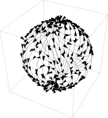
Ideally, the front of spherical surface should be partially transparent so that the flow line at the rear end can be visualized at the same time.

Answer 1

An alternative way to post-process the StreamPlot output into a Graphics3D object using @user18792's trick:

sp = StreamPlot[{Cot[θ] Cos[ϕ], -Sin[ϕ]}, {ϕ, -π, π}, {θ, 0, π}, StreamColorFunction -> Hue, 
   ImageSize -> 400];

sp3d = Graphics3D[sp[[1]] /. Arrow[z_] :> 
       Arrow[z /. {x_Real, y_Real} :> {Cos[x] Sin[y], Sin[y] Sin[x],  Cos[y]}], ImageSize -> 400];
Row[{sp, sp3d}, Spacer[5]]

To add a semi-transparent Sphere:

Graphics3D[{sp[[1]] /. Arrow[z_] :> 
             Arrow[z /. {x_Real, y_Real} :> {Cos[x] Sin[y], Sin[y] Sin[x], Cos[y]}], 
            Opacity[.5], Sphere[]}, ImageSize -> 400]

Answer 2

gr = Normal@StreamPlot[{Cot[θ] Cos[ϕ], -Sin[ϕ]}, {ϕ, -π, π}, {θ, 0, π}, 
  StreamColorFunction -> Hue];

Graphics3D[Cases[gr, _Arrow, Infinity] /. 
  {x_Real, y_Real} :> {Cos[x] Sin[y], Sin[y] Sin[x], Cos[y]}]