How to connect discrete points and make them become continuous curve?

Question

Given that I have two variables $\theta,t$, for the varible $t$, $\theta$ always owns several values. Namely, $$\{t,\theta_1,\theta_2,\theta_3,\theta_4...\}$$ where $t$ in the interval$[0,1]$ and $\theta$ in the interval$[0,2\pi]$

My sample data

originalData=
{{0,2.99939,6.16435},{0.010101,3.03635,6.19686},{0.020202,3.07484,6.22946}, 
 {0.030303,3.11493,6.26213},{0.040404,0.011674,3.15666}, 
 {0.0505051,0.0444528,3.20004},{0.0606061,0.0772844,3.24504},
 {0.0707071,0.110179,3.29156},{0.0808081,0.143159,3.33945},
 {0.0909091,0.176258,3.38851},{0.10101,0.209527,3.43847},{0.111111,0.243035,3.48904},
 {0.121212,0.276879,3.53988},{0.131313,0.311186,3.59066},{0.141414,0.346126,3.64109},
 {0.151515,0.381932,3.69088},{0.161616,0.418919,3.73981},{0.171717,0.457536,3.78768},
 {0.181818,0.498437,3.83436},{0.191919,0.54263,3.87976},{0.20202,0.591793,3.92382},
 {0.212121,0.649054,3.96653},{0.222222,0.7215,4.00787},
 {0.232323,1.79066,1.4441,0.834008,4.0479},{0.242424,2.04691,4.08662},
 {0.252525,2.17701,4.12412},{0.262626,2.27155,4.16044},
 {0.272727,2.3473,4.19565},{0.282828,2.41109,4.22982},{0.292929,2.46649,4.26302},
 {0.30303,2.51566,4.29532},{0.313131,2.56,4.3268},{0.323232,2.60048,4.35752},
 {0.333333,2.63783,4.38756},{0.343434,2.67258,4.41699},{0.353535,2.70514,4.44588},
 {0.363636,2.73583,4.47429},{0.373737,2.76491,4.5023},{0.383838,2.79261,4.52997},
 {0.393939,2.81908,4.55739},{0.40404,2.84448,4.58461},{0.414141,2.86894,4.61171},
 {0.424242,2.89255,4.63878},{0.434343,2.91541,4.66589},{0.444444,2.9376,4.69313}, 
 {0.454545,2.95918,4.7206},{0.464646,2.9802,4.74841},{0.474747,3.00073,4.77666},
 {0.484848,3.02081,4.8055},{0.494949,3.04048,4.83508},{0.505051,3.05977,4.86559},
 {0.515152,3.07872,4.89726},{0.525253,3.09736,4.93036},
 {0.535354,3.1157,0.308209,0.214389,4.96529},
 {0.545455,3.13379,0.428984,0.0480804,5.0025},
 {0.555556,0.485269,6.22645,5.04269,3.15163},  
 {0.565657,0.526307,6.13285,5.08687,3.16925},
 {0.575758,0.55954,6.0414,5.13667,3.18666},
 {0.585859,0.587877,5.94624,5.19502,3.20387},
 {0.59596,0.612803,5.83937,5.26845,3.22092},
 {0.606061,0.635191,5.69654,5.38031,3.2378},{0.616162,0.655606,3.25452},
 {0.626263,0.674433,3.27111},{0.636364,0.691951,3.28758},{0.646465,0.708367,3.30392},
 {0.656566,0.72384,3.32015},{0.666667,0.738494,3.33628},{0.676768,0.75243,3.35231},
 {0.686869,0.765729,3.36826},{0.69697,0.778458,3.38412},{0.707071,0.790675,3.3999},
 {0.717172,0.802427,3.41561},{0.727273,0.813756,3.43125},{0.737374,0.824695,3.44683},
 {0.747475,0.835277,3.46235},{0.757576,0.845527,3.4778},{0.767677,0.85547,3.4932},
 {0.777778,0.865127,3.50855},{0.787879,0.874516,3.52384},{0.79798,0.883655,3.53909},
 {0.808081,0.892558,3.55428},{0.818182,0.901239,3.56942},{0.828283,0.90971,3.58452},
 {0.838384,0.917984,3.59956},{0.848485,0.92607,3.61456},{0.858586,0.933978,3.6295},
 {0.868687,0.941717,3.64439},{0.878788,0.949295,3.65923},{0.888889,0.956718,3.67401},
 {0.89899,0.963995,3.68873},{0.909091,0.971132,3.70339},{0.919192,0.978135,3.71798},
 {0.929293,0.985008,3.73251},{0.939394,0.991759,3.74697},{0.949495,0.998391,3.76135},
 {0.959596,1.00491,3.77566},{0.969697,1.01132,3.78988},{0.979798,1.01762,3.80402},
 {0.989899,1.02382,3.81806},{1.,1.02993,3.83201}};

My goal

I would like to plot independent curves according these discrete points in one graphic.

My trial

Firstly, I visualize these discrete points and show them in one graphic:

 Data1 = Thread@{originalData[[All, 1]], originalData[[All, 2]]};
 Data2 = Thread@{originalData[[All, 1]], originalData[[All, 3]]};
 middle = Cases[originalData, {_, _, _, _, _}];
 Data3 = Thread@{middle[[All, 1]], middle[[All, 4]]};
 Data4 = Thread@{middle[[All, 1]], middle[[All, 5]]};

 Show[
  ListPlot[#1, PlotStyle -> {#2, PointSize[Small]}] & @@@
   (Thread@{{Data1, Data2, Data3, Data4}, {Red, Blue, Black, Green}}),
   AxesOrigin -> {0, -1}, ImageSize -> 700, 
   PlotRange -> {{0, 1}, {-1, 7}},
   GridLines -> {{}, {0, 2 \[Pi]}}, AxesStyle -> Arrowheads[.02],
   GridLinesStyle -> Directive[RGBColor[1, 0, 1], Dashed],
   AxesLabel -> (Style[#, 15, Red, Italic, 
   FontFamily -> "Helvetica"] & /@ {"t", "\[Theta]"})]

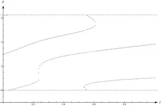
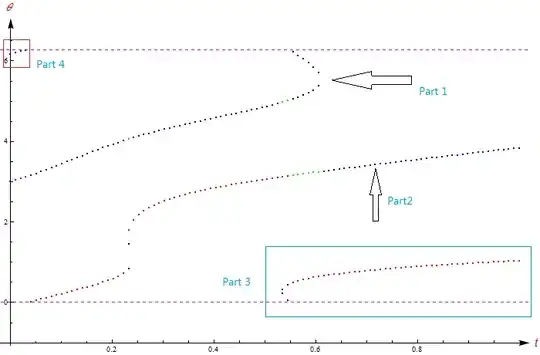
By the visualizstion of ListPlot and Show, I know that there are 4 part(Part 1,Part 2,Part 3,Part 4) subpictures in this graphic.

enter image description here

My question(difficulty)

1,Is it possible to connect the the disrete points of Part $i$.Namely, make the Part $i$ become a continuous curve?

2,Now I have no idea to solve this problem, so if possible, can someone give some suggestions (algorithm or hint)? Thanks in advance:-)

You could use Nearest or similar to stitch your point sets together. Other possibly (?) useful functions: FindCurvePath and FindShortestTour. — Yves Klett, Jan 04 '15 at 08:52

Yi Wang · Accepted Answer · 2015-01-11T08:03:22.437

20

Method 1: FindCurvePath (as mentioned by Yves Klett). This method is simple, but unfortunately, there are small issues (as shown in plots), that the curves are not identified perfectly.

arrayData = 
  Flatten[Function[{lst}, {First @ lst, #} & /@ Rest[lst]] /@ 
    originalData, 1];

curvesPosition = FindCurvePath[arrayData];

ListPlot[curves = 
  arrayData[[curvesPosition[[#]]]] & /@ Range@Length@curvesPosition, 
 Joined -> True, PlotMarkers -> None]

enter image description here

Method 2: Code to separate curves by hand:

The list arrayData converts originalData into the form {{t1, θ1}, {t2, θ2}, ...}. This form is easier for processing.

arrayData = 
  Flatten[Function[{lst}, {First @ lst, #} & /@ Rest[lst]] /@ 
    originalData, 1];

Because we plan to measure EuclideanDistance later, we first normalize the data. After splitting the data into segments, we shall restore the standard deviation.

SD = StandardDeviation[arrayData];
applySD = {#1/SD[[1]], #2/SD[[2]]} &;
restoreSD = {#1 * SD[[1]], #2 * SD[[2]]} &;

normData = applySD @@@ arrayData;

To avoid curves breaking in the middle, we shall need to find starting points of a a curve. The function findStart does this job. The best guess starting point A is the point such that the two nearest points to A (denoted by B and C) point to closest directions, i.e. ∠BAC is smallest. If the points are dense enough, ∠BAC should be close to 0 for starting points, and close to π for a point in the middle of a segment.

findStart[lst_]:= Module[{near1, near2, angle, best, bestAngle = Infinity},
    Do[
        If[Length @ lst <= 2, Return[lst[[1]]]];
        {near1, near2} = Nearest[lst, elem, 3][[2;;]]; (* exclude elem itself *)
        angle = VectorAngle[near1-elem, near2-elem];
        If[angle < bestAngle, best = elem; bestAngle = angle]
    , {elem, lst}];
    best]

The moveStep is the major function to do the work. moreStep[{lst, new}] acts as follows:

Find the nearest point to the last element of new in lst. If the point is near (there is a parameter to define near, 0.5 in the code), move the nearest point from lst to new. If the nearest point is too far away (i.e. not on the current segment), save the current segment and reset the new list.

Note that the list that the OP gives is ordered in t. If it is not the case, one should sort the list by t. Otherwise, a segment may be broken into two from the middle.

moveStep = Function[{input},Module[{elem,neighbor,lst,new},
    lst = First@input;
    new = Last@input;
    If[new=!={}, elem=new[[-1]], elem = findStart @ lst];
    neighbor=Nearest[lst,elem][[1]];
    If[EuclideanDistance[elem,neighbor]>0.5, 
        AppendTo[segments,new];
        {lst, {}}
        ,{DeleteCases[lst,neighbor], Append[new,neighbor]}]]];

Then we shall apply multiple steps using Nest. Each step moves one element. Thus the number of steps to nest is length of arrayData.

segments = {};
test = NestWhile[moveStep, {normData, {}}, #[[1]] =!= {} &];
AppendTo[segments, Last@test];

Restore standard derivation, and plot the result.

result = Apply[restoreSD, segments, {2}];

ListPlot[result, Joined -> True, PlotMarkers -> None]

enter image description here

edited Jan 11 '15 at 08:03

answered Jan 04 '15 at 11:51

Yi Wang

7,347
4
28
38

1

Nice answer!I am reading this to understand your program!Thanks a lot:-) – xyz Jan 05 '15 at 06:16
1

Dear Yi Wang, I cannot understand the code If[neighbor===elem, neighbor = Nearest[DeleteCases[lst, neighbor], elem][[1]]];in the function moveStep. Could you explain it to me? In addition, I'd like to know that why the data need be normalized? Thanks !:-) – xyz Jan 06 '15 at 02:13
1

@ShutaoTang : After looking at the code again, I apologize that there were a few problems. (1) As you points out, this If[...] statement is confusing and not necessary. To keep things consistent, DeleteCases[lst,neighbor] is used for both cases at the end of moveStep. (2) I noted that in the previous version, "⊂" shaped curve cannot be identified nicely, because it cannot guess the start point of "⊂" shaped curve. I added findStart function to find starting point of a curve more carefully. – Yi Wang Jan 06 '15 at 07:45
Also, it appears a bit stupid to use Do loop to find minimal value. MinimalBy should be the one to use. But considering that MinimalBy is a new function in version 10, I did not use it for compatibility reason. I believe there are some other bad practices as well because I am feeling that I am not writing functional code (with a similar experience to writing in C with a handy math library) when coding it up. – Yi Wang Jan 06 '15 at 07:58
In the morning,@Yi Wang to understand the purpose of that code, I deleted that code(If[]) then I got a closely similar result. – xyz Jan 06 '15 at 08:02
1

The data is normalized because, otherwise, calculating EuclideanDistance in the vertical piece "|" and the horizontal piece "-" of a curve cannot give comparable result. – Yi Wang Jan 06 '15 at 08:03
When I encoutered this problem a week ago firstly,@Yi Wang I didn't have any idea to deal with it. So I am very happy and honor to get your help. In addition, I am used writing functional programming in MMA, but the *algorithm* in your code is very significant and it is worth studying：) – xyz Jan 06 '15 at 08:11
@ShutaoTang : Nice to hear that you like it :) – Yi Wang Jan 06 '15 at 08:17
3

For speed improvement I would suggest precomputing nf=Nearest[list] (outside moveStep) and then using nf[elem] subsequently. I think it will be faster to pass the NearestFunction into the subroutine than to recompute it every time. – Daniel Lichtblau Jan 06 '15 at 15:53
Another idea is that a point will "usually" have but two nearest neighbors. When it does not, the "crossings" can often be detected simply by deciding which pairs have similar one-sided directions (or just by taking non-adjacent points for each neighbor pair). This will need work in cases where two curves approach but do not cross, or when neighbors of a crossing also claim to have more than two neighbors. I would expect that numerical derivative approximations will be needed to sort out such cases. – Daniel Lichtblau Jan 06 '15 at 15:58
@DanielLichtblau : Thanks a lot for the comments! (1) Note that lst is modified each time moveStep is called, at DeleteCases[lst,neighbor]. Thus I cannot pre-compute a list before calling moveStep. The performance of the code should be very bad. Luckily the list that the OP gives is not too large. For very large lists, we may need to reconsider the algorithm. (2) That's a good point! I haven't considered the crossing case. That would be similar to the case of searching for start point of the segment, by consider angles among nearest points. – Yi Wang Jan 06 '15 at 19:59
Great work! I think the findStart function may need a small correction: the If[Length @ lst <= 2, Return[lst[[1]]]]; statement should appear before the Do loop; otherwise the Return exits the Do loop but not the function itself. – Simon Rochester Mar 16 '15 at 23:04
@SimonRochester: Good point! I think you are right but I am a bit busy now and will test that later. (The code nevertheless still works. Probably that If is not necessary?) – Yi Wang Mar 17 '15 at 00:45
It's only a problem if you happen to have one or two points left over after collecting all of the other segments. Then it throws an error, which is how I noticed it. So it's usually not necessary, but occasionally crucial... – Simon Rochester Mar 17 '15 at 05:52

score 13 · Answer 2 · edited May 23 '15 at 03:06

One can use the periodicity over $\theta$ and add one periodic copy of the data. In this case FindCurvePath works much better. I also add an interpolation of the result

arrayData = Flatten[Thread@{#, Join[{##2}, {##2} + 2 π]} & @@@ originalData, 1];
curvesPosition = FindCurvePath@arrayData;
{t, θ} = Interpolation@Transpose@{Range[0., 1, 1/(Length@# - 1)], #} & /@ 
      Transpose@arrayData[[#]] & /@ curvesPosition // Transpose;

ParametricPlot[Evaluate@Table[{t[[i]][ξ], θ[[i]][ξ]}, {i, Length@t}], {ξ, 0, 1}, 
 AspectRatio -> 1/GoldenRatio, PlotRange -> {{0, 1}, {0, 4 π}}]

plot of data

Let's select only full curves and plot them by $\bmod 2\pi$. Now we explicitly see that there are only two branches:

ParametricPlot[{{t[[1]][ξ], Mod[θ[[1]][ξ], 2 π]}, 
  {t[[2]][ξ], Mod[θ[[2]][ξ], 2 π]}}, {ξ, 0, 1}, 
 AspectRatio -> 1/GoldenRatio, PlotRange -> {{0, 1}, {0, 2 π}}]

plot with two branches

How to connect discrete points and make them become continuous curve?

My question(difficulty)

2 Answers2

Linked