Number of divisors visualized with the QPochhammer function, how to improve performance of code?

Question

I have this code that is originally Jeffrey Stopple's code for the Riemann zeta function in the complex plane. Because I discovered yesterday that the number of divisors can be generated with the $q$-Pochhammer symbol (QPochhammer), and since Mathematica shows a plot of QPochhammer, I thought that plotting it would be fun.

Here is the code that needs improvement:

Show[Graphics[RasterArray[
   Table[Hue[Mod[3 Pi/2 + 
        Arg[Sum[(s + I t)^(n - 1)*(QPochhammer[(s + I t)^(n + 1), (s + I t)]/
             QPochhammer[(s + I t)^(n), (s + I t)]), {n, 1, 100}]], 
       2 Pi]/(2 Pi)], {t, -1.1, 1.1, .05}, {s, -1.1, 1.1, .05}]]], 
 AspectRatio -> Automatic]

And the code for the number of divisors:

CoefficientList[
 Series[Sum[
   x^(n - 1)*(QPochhammer[x^(n + 1), x]/QPochhammer[x^(n), x]), {n, 1,
     104}], {x, 0, 103}], x] (*_ Mats Granvik_,Jan 03 2015*)

1, 2, 2, 3, 2, 4, 2, 4, 3, 4, 2, 6, 2, 4, 4, 5, 2, 6, 2, 6, 4, 4, 2, 8, 3, 4, 4,
6, 2, 8, 2, 6, 4, 4, 4, 9, 2, 4, 4, 8, 2, 8, 2, 6, 6, 4, 2, 10, 3, 6, 4, 6, 2, 8,
4, 8, 4, 4, 2, 12, 2, 4, 6, 7, 4, 8, 2, 6, 4, 8, 2,...

The plot from the first program that I would like to improve:

Already if someone could post a plot with higher resolution, I would be glad. My computer is rather old.

Answer 1

It looks like you want to plot the phase-only information of a complex function. Using the following helper functions for plotting the phase-only information complex functions:

hue = Compile[{{z, _Complex}}, {Mod[3 π/2 + Arg[z], 
      2 π]/(2 π), 1, If[Abs[z] > 10^-3, 1, 0]}, 
   CompilationTarget -> "C", RuntimeAttributes -> {Listable}];
ComplexPlotC[f_, {x0_, x1_, δx_}, {y0_, y1_, δy_}] := 
  Image[hue[
     f[Outer[Complex, Range[x0, x1, δx], 
       Range[y1, y0, -δy]]]]\[Transpose], ColorSpace -> Hue, 
   Magnification -> 1];
CCompileC[expr_] := 
  Compile[{{z, _Complex}}, Evaluate[expr], CompilationTarget -> "C", 
   RuntimeAttributes -> {Listable}];

You can then compile your function and plot it (I'll only sum 10 terms, rather than 100, as using 100 would take quite a long time):

func = CCompileC[
   If[Abs[z] >= 0.999, 0, 
    Sum[z^(n - 1)*(QPochhammer[z^(n + 1), z]/
        QPochhammer[z^(n), z]), {n, 1, 10}]]];
ComplexPlotC[func, {-1 + 10^-6 RandomReal[], 1, 
  0.003}, {-1 + 10^-6 RandomReal[], 1, 0.003}]

which gives the following:

Here is a 100-term sum picture (open in separate tab to see slightly larger picture):

Answer 2

As this is a special-functions question, I feel justified in using a bit of heavy artillery. Here goes nothing...

In effect, what the OP seems to want to do is to evaluate

$$\sum_{n=1}^\infty \frac{(q^{n+1};q)_\infty}{(q^n;q)_\infty} q^{n-1}$$

(where $(a;q)_n$ is the $q$-Pochhammer symbol) by approximating it with its partial sums. However, there is a more streamlined expression for this function.

Using, for instance, formula 12 in the MathWorld page I linked to, we have

$$\begin{align*}\sum_{n=1}^\infty \frac{(q^{n+1};q)_\infty}{(q^n;q)_\infty} q^{n-1}&=\frac{(q^2;q)_\infty}{(q;q)_\infty}\sum_{n=0}^\infty \frac{\frac{(q;q)_\infty}{(q^{n+1};q)_\infty}}{\frac{(q^2;q)_\infty}{(q^{n+2};q)_\infty}} q^n\\&=\frac1{(q;q)_1}\sum_{n=0}^\infty \frac{(q;q)_n}{(q^2;q)_n} q^n\\&=\frac1{1-q}\sum_{n=0}^\infty \frac{(q;q)_n (q;q)_n}{(q^2;q)_n}\frac{q^n}{(q;q)_n}\end{align*}$$

and the infinite sum can now be recognized as the $q$-hypergeometric function $$\frac1{1-q}\,{}_2\phi_1\left({{q,q}\atop{q^2}}\mid q,q\right)$$

or in Mathematica syntax, QHypergeometricPFQ[{q, q}, {q^2}, q, q]/(1 - q).

Another expression is derived by noting that

$$\frac{(q;q)_n}{(q^2;q)_n}=\frac{1-q}{1-q^{n+1}}$$

Using this identity instead in the derivation above yields

$$\begin{align*}\frac1{1-q}\sum_{n=0}^\infty \frac{(q;q)_n}{(q^2;q)_n} q^n&=\frac1{q}\sum_{n=1}^\infty \frac{q^n}{1-q^n}\end{align*}$$

i.e., a Lambert series, which is expressible in terms of the $q$-digamma function (compare the definitions)

$$\frac{\psi_q(1)+\log(1-q)}{q\log q}$$

or (QPolyGamma[1, q] + Log[1 - q])/(q Log[q]) in Mathematica syntax.

We now have two alternative expressions to choose from. The $q$-digamma function is faster to evaluate (at least in the tests I did), but the $q$-hypergeometric expression does not have the removable singularity at the origin.

If we are to use the $q$-digamma function expression, then, this precludes us from an Image[]-based approach such as the one in the OP and the other answer. We could use DensityPlot[] (since it does not visibly complain about singularities) with an appropriate RegionFunction setting, but a better way would be to use another classical technique, this time from Schwarz and Christoffel.

To be precise, what I'll do here is to use the conformal map from the unit square to the unit disk within DensityPlot[] and then perform an ImageForwardTransformation[] (like in the one done here) to finally obtain the image on the unit disk. As mentioned in that other answer, the appropriate mapping function is JacobiSN[z, 1/2] JacobiDC[z, 1/2]. The built-in Jacobi elliptic functions are a bit slow for image transformation purposes, so I have written a compiled function that evaluates this mapping for complex arguments:

sdc = With[{c1 = 1./2678, c2 = 1101., c3 = 110.2, c4 = 5677./60, 
            c5 = 1577., c6 = 1479., c7 = 21739./60, d1 = 1./338, d2 = 51., 
            d3 = 1./15, d4 = 1709., d5 = 262.25, d6 = 287., d7 = 0.2, 
            d8 = 1591./3, d9 = 102.75},
           Compile[{{z, _Complex}}, Module[{dc, k, s, zs, zs2},
                    k = If[z == 0., 0, Max[0, Ceiling[Log2[4. Abs[z]]]]];
                    zs = z/(2^k); zs2 = (zs/2)^2;
                    {s, dc} = {(zs (1. - c1 zs2 (c2 + zs2 (c3 - c4 zs2))))/
                               (1. + c1 zs2 (c5 - zs2 (c6 - c7 zs2))),
                               (1. + d1 zs2 (d2 + d3 zs2 (d4 + d5 zs2)))/
                               (1. - d1 zs2 (d6 + d7 zs2 (d8 + d9 zs2)))};
                    Do[{s, dc} = {(2. s dc)/(1. + s^2 dc^2),
                                  (dc^2 - 0.5 s^2)/(1. - s^2 dc^2)}, {k}];
                    s dc], RuntimeAttributes -> {Listable}]]

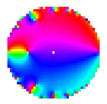
We now generate the image in two stages. First, here's the "raw" DensityPlot[]:

With[{ω = N[3 Beta[5/4, 5/4]/2], ε = 1/100},
     sqrimg = DensityPlot[With[{q = sdc[ω (x + I y)]}, 
                               Arg[(QPolyGamma[1, q] + Log[1 - q])/(q Log[q])]],
                          {x, -1 + ε, 1 - ε}, {y, -1 + ε, 1 - ε}, 
                          ColorFunction -> (Hue[Mod[#/(2 π) + 3/4, 1]] &), 
                          ColorFunctionScaling -> False, Frame -> None,
                          ImageSize -> Large, MaxRecursion -> 1,
                          PlotPoints -> 95, PlotRangePadding -> None]]

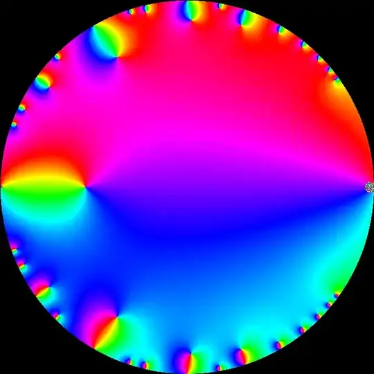
Some features should already be recognizable in this distorted image. Now, undo the Schwarz-Christoffel distortion like so:

With[{ω = N[3 Beta[5/4, 5/4]/2]}, 
     ImageForwardTransformation[sqrimg, With[{z = ω (#[[1]] + I #[[2]])},
                                Through[{Re, Im}[sdc[z]]]] &, Background -> 1.,
                                DataRange -> {{-1, 1}, {-1, 1}}]]

Beautiful. If need be, you can always increase the setting for PlotPoints and MaxRecursion, but the picture already looks reasonably good to me. (Note that the jittery portion near $q=1$ in the other images posted is completely absent.)