I need a function for a series of joined slopes and my solution feels a bit kludgy. Is there a better way?
A list of pairs of transition points and slopes:
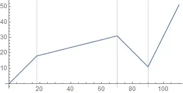
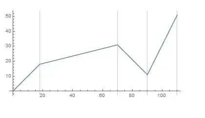
dat = {{0, 0}, {18, 1}, {70, 1/4}, {90, -1}, {110, 2}};
Build a function:
ClearAll[f]
f[0] = 0;
Cases[
  Partition[dat, 2, 1],
  {{lo_, _}, {hi_, slope_}} :>
    (f[x_ /; x <= hi] := f[lo] + slope (x - lo))
];
Plot it:
Plot[f[x], {x, 0, 110}, AspectRatio -> Automatic, GridLines -> {{18, 70, 90}, None}]
The input format (dat) is arbitrary and could possibly be better too.
Performance
There are presently three answers using Interpolation including my own. Speed of evaluation of the InterpolatingFunction appears to be the same in each case. Here is a comparison of the speed of generation in 10.1.0 under Windows. I shall cheat for my method by using a pure function (g2) which trades clarity for speed. (Spoiler: it still doesn't win.)
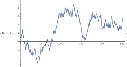
SeedRandom[1]
dat = {Accumulate @ RandomReal[{0, 1}, 1000], RandomReal[{-1, 1}, 1000]}\[Transpose];
RepeatedTiming[
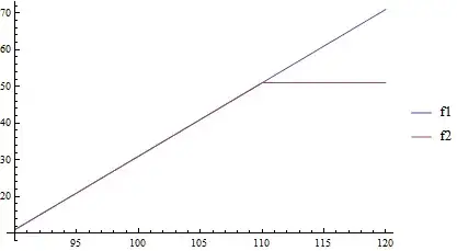
f1[x_] = Integrate[Interpolation[dat, InterpolationOrder -> 0][x], x];
]
{0.00215, Null}
g2 = {#2[[1]], #[[2]] + (#2[[1]] - #[[1]]) #2[[2]]} &;

RepeatedTiming[
  f2 = Interpolation[FoldList[g2, dat], InterpolationOrder -> 1];
]
{0.00145, Null}
RepeatedTiming[
  x = dat[[;; , 1]];
  y = {#}~Join~(# + Accumulate[Differences[x] dat[[2 ;;, 2]]]) &@dat[[1, 2]];
  f3 = Interpolation[Transpose[{x, y}], InterpolationOrder -> 1];
]
{0.000972, Null}
So it seems Algohi's code is fastest at less than half the time of Integrate.
(His answer deserves more votes!)


datformat the pairs {v, s} should be read as "use slope s up to value v" -- the{0, 0}what just added to make my kludgy function work. – Mr.Wizard Jan 09 '15 at 22:14f[x_] := ... + 0.1. Just curious. – Mr.Wizard May 25 '15 at 11:32