Define a function with variables linked implicitly

Question

I would like to define a function $f(x,y)$, with the variables x and y linked by an equation implicitly, so $f(x,y)=f(x(y),y)=f(y)$.

Eventually I would like to draw a graph with $f(x(y),y)$ being the output and $y$ being the input.

One example is $f(x,y)=x+y$ and $exp(xy)=y$. How can I do it?

try ClearAll[f, g, h]; f[x_, y_] := x + y; g[y_] := Log[y]/y; h[y_] := f[g[y], y] — kglr, Feb 09 '15 at 03:47
Thanks. What if the relationship is more complicated, say y=cos(xy)+exp(x)+exp(y)? That is, I cannot rearrange the variables to define g[y_]? — fanshenry, Feb 09 '15 at 04:02

score 4 · Answer 1 · answered Feb 09 '15 at 05:54

4

f[x_, y_] := x + y
g[x_, y_] := Exp[x y] - y;
ParametricPlot[{y, f[x, y]}, {x, -5, 5}, {y, -5, 5}, 
 MeshFunctions -> {Function[{a, b, x, y}, g[x, y]]}, Mesh -> {{0}}, 
 PlotStyle -> None, BoundaryStyle -> None, 
 MeshStyle -> {{Opacity[1], Thick, Black}}, PlotRange -> All, 
 Frame -> False]

enter image description here

answered Feb 09 '15 at 05:54

Thanks. What does MeshFunctions -> {Function[{a, b, x, y} stand for? To follow up my question, how can I define the function f(x(y),y)? I would like to use the function to do more. – fanshenry Feb 09 '15 at 06:06
@Rahul +1 very nice trick. – Basheer Algohi Feb 09 '15 at 06:56
@fanshenry: Sorry, I took "Eventually I would like to draw a graph" to mean that drawing the graph was your end goal. To define the function itself, you can try using Solve or NSolve or use Michael E2's method. When I have some more time, I'll edit my answer to explain the use of MeshFunctions, but in the meantime you could look at the documentation. – Feb 09 '15 at 17:00

kglr · Answer 2 · 2015-02-09T10:04:59.463

My preferred method would be using @rahul's Mesh trick. You can also use the option Exclusions as follows:

f[x_, y_] := x + y
g[x_, y_] := Exp[x y] - y;
ParametricPlot[{y, f[x, y]}, {x, -5, 5}, {y, -5, 5}, 
 Frame -> False, PlotRange -> All, BoundaryStyle -> None, Mesh -> None, PlotStyle -> None,
 Exclusions -> {g[x, y] == 0}, 
 ExclusionsStyle -> Directive[Thick, Opacity[1], EdgeForm[Blue], Blue, Antialiasing -> True]]

enter image description here

Note: Unlike @rahul's method which produces a single Line primitive, this method produces Polygons.

score 2 · Accepted Answer · edited Apr 13 '17 at 12:56

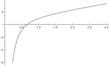
To me the question is more about calculating the function than generating the plot.

Given an equation that cannot be solved symbolically, we can approximate the implicit function with NDSolve. (There are several examples on this site., e.g., Getting an InterpolatingFunction from a ContourPlot, Plotting implicitly-defined space curves.)

implicitFunction::usage = "implicitFunction[equation, {y, y0}, {x, x0, start, end}]";
Begin["implicitFunction`"];
implicitFunction[eq_, {f_Symbol, f1_?NumericQ},
     {x_Symbol, x1_?NumericQ, xmin_?NumericQ, xmax_?NumericQ}] :=
  Block[{f0, xt},
   f0 = f /. FindRoot[eq /. x -> x1, {f, f1}];
   NDSolveValue[
     {eq /. {x -> x[xt], f -> f[xt]}, x'[xt] == 1, f[x1] == f0, x[x1] == x1},
     f, {xt, xmin, xmax}]
   ];
End[];

We need to propose a domain for our approximation and approximate initial values for x and y. FindRoot is used to refine the initial value for the function x.

eq1 = Exp[x y] == y;
ξ = implicitFunction[eq1, {x, 0}, {y, 1, -3, 3}];

NDSolveValue::ndsz: At implicitFunction`xt == 1.111713753522611`*^-16, step size is effectively zero; singularity or stiff system suspected. >>

The warning just means that NDSolve has computed the domain for us:

ξ["Domain"]
(*  {{1.11171*10^-16, 3.}}  *)

Plot[ξ[y] + y, Evaluate @ Flatten[{y, ξ["Domain"]}]]

Mathematica graphics

One could further process the result by wrapping the interpolating function with FindRoot. For this we need to add the attribute HoldAll. The following could be incorporated as a second definition of implicitFunction, but here I'll simply make a second definition. The only advantage is when a more accurate value is needed. One can take advantage of the FindRoot options.

SetAttributes[implicitFunction2, HoldAll];
implicitFunction2[eq_, f_Symbol, x_Symbol, init_: (0 &), opts : OptionsPattern[FindRoot]][x1_?NumericQ] := 
  Block @@ Hold[{f, x}, f /. FindRoot[eq /. x -> x1, {f, init[x1]}]];

The init function supplies the initial value for the root. We can use the NDSolve interpolating function to do that (at least within its domain).

ξ2 = implicitFunction2[eq1, x, y, ξ];
Plot[ξ2[y] + y, Evaluate@Flatten[{y, ξ["Domain"]}]]
(* plot looks the same as above *)

This form also works with the default init, but that is because the equation is easy to solve from any starting point.

ξ2 = implicitFunction2[eq1, x, y];

Of course, it's slower than just using ξ.

Basheer Algohi · Answer 4 · 2015-02-09T07:47:30.347

1

If post processing is acceptable then:

ContourPlot[Exp[x y] == y, {x, -5, 5}, {y, -5, 5}, Frame -> False, 
  Axes -> True] /. 
 GraphicsComplex[a_, b___] :> 
  GraphicsComplex[({#2, #2 + #1} &) @@@ a, b]

enter image description here

edited Feb 09 '15 at 07:47

answered Feb 09 '15 at 07:38

Basheer Algohi

19,917
1
31
78

score 1 · Answer 5 · answered Feb 09 '15 at 08:51

You can also eliminate the implicit dependency by using Solve, e.g.:

res=Solve[Exp[x y]==y,x][[1,1]]/.C[1]->0

and apply the result to the output function:

x+y/.res

or combine the steps into one:

x+y/.Solve[Exp[x y]==y,x][[1,1]]/.C[1]->0
(* y+Log[y]/y *)

This way, you end with the desired function of y only, may use standard plotting, and of course any other analytics, differentiate, …

Plot[Evaluate[x+y/.Solve[Exp[x y]==y,x][[1,1]]/.C[1]->0],{y,-5,5}]

y+Log[y]/y

Define a function with variables linked implicitly

5 Answers5

Linked