We are asked to maximize and minimize $f(x,y)=4xy$, given the constraint $4x^2+y^2=8$, using the Lagrange Multiplier method. First, I enter the functions f and g.
f = 4 x*y;
g = 4 x^2 + y^2 - 8;
Then I solve using the Lagrange Multiplier method.
sols = Solve[{Grad[f, {x, y}] == λ Grad[g, {x, y}],
   g == 8}, {x, y, λ}]
Which gives this output.
   {{x -> -1, y -> -2, λ -> 1}, {x -> -1,
      y -> 2, λ -> -1}, {x -> 1,
      y -> -2, λ -> -1}, {x -> 1, y -> 2, λ -> 1}}
I can then create the points to investigate.
{x, y} /. sols
Which gives this output.
{{-1, -2}, {-1, 2}, {1, -2}, {1, 2}}
Now I can evaluate f at each point.
f /. sols
Which gives this output.
{8, -8, -8, 8}
So, I have maximum values of 8 at the points $(-1,-2)$ and $(1,2)$, and minimum values of $-8$ at the points $(-2,2)$ and $(1,-2)$. Now, this can be visualized with the following image.
ContourPlot[f, {x, -2, 2}, {y, -3, 3},
 Contours -> Range[-10, 10],
 Mesh -> {{0}}, MeshFunctions -> Function[{x, y}, g],
 MeshStyle -> Directive[Thick, Yellow],
 Epilog -> {Red, PointSize[Large], Point[{x, y}] /. sols}]

Now, my question. I want to use the Lagrange multiplier technique to maximize $f(x,y,z)=xyz$ subject to the constraint $x^2+10y^2+z^2=5$.
f = x y z;
g = x^2 + 10 y^2 + z^2;
sols = Solve[{Grad[f, {x, y, z}] == λ Grad[g, {x, y, z}],
    g == 5}, {x, y, z, λ}];
{x, y, z} /. sols
Gives the following output.
{{0, 0, -Sqrt[5]}, {0, 0, Sqrt[5]}, {0, -(1/Sqrt[2]), 0}, {0, 1/Sqrt[
  2], 0}, {-Sqrt[(5/3)], -(1/Sqrt[6]), -Sqrt[(5/3)]}, {-Sqrt[(5/
   3)], -(1/Sqrt[6]), Sqrt[5/3]}, {-Sqrt[(5/3)], 1/Sqrt[
  6], -Sqrt[(5/3)]}, {-Sqrt[(5/3)], 1/Sqrt[6], Sqrt[5/3]}, {Sqrt[5/
  3], -(1/Sqrt[6]), -Sqrt[(5/3)]}, {Sqrt[5/3], -(1/Sqrt[6]), Sqrt[5/
  3]}, {Sqrt[5/3], 1/Sqrt[6], -Sqrt[(5/3)]}, {Sqrt[5/3], 1/Sqrt[6],
  Sqrt[5/3]}, {-Sqrt[5], 0, 0}, {Sqrt[5], 0, 0}}
And we can evaluate f at each of these points.
f /. sols

{0, 0, 0, 0, -(5/(3 Sqrt[6])), 5/(3 Sqrt[6]), 5/(
 3 Sqrt[6]), -(5/(3 Sqrt[6])), 5/(
 3 Sqrt[6]), -(5/(3 Sqrt[6])), -(5/(3 Sqrt[6])), 5/(3 Sqrt[6]), 0, 0}
So it appears that I have a maximum value of $\dfrac{5}{3\sqrt6}$ at four separate points and a minimum value of $-\dfrac{5}{3\sqrt6}$ at four separate points.
So, it appears I can do this part. The part I need help with is the image. Is it possible to produce contour surfaces of f and show where the constraint $g(x,y,z)=5$ touches a level surface of f at the minimum and maximum points?
Or, one image that shows touches at the maximum points and a second image that shows touches at the minimum points?
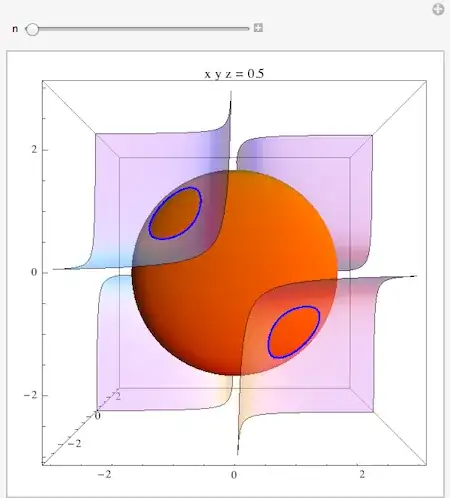
ContourPlot3Dwith suitablezrange spec, and likewise addzto theMeshFunctionssetting. – Daniel Lichtblau Mar 27 '15 at 16:38