I want to form the function $h=f-\lambda_{1}g_{1}-\lambda_{2}g_{2}$ where $f$ is the function to optimize subject to the constraints $g_{1}=0$ and $g_{2}=0$ so that I can solve the first partial derivatives with respect to $\lambda_{1}$ and $\lambda_{2}$. Can someone get me started using $f(x,y,z)=xy+yz$ subject to the constraints $x^2+y^2-2=0$ and $x^2+z^2-2=0$?
Asked
Active
Viewed 1.0k times
21
J. M.'s missing motivation
- 124,525
- 11
- 401
- 574
Logan
- 517
- 1
- 6
- 15
3 Answers
31
We define the function f and multiple constraint functions g1, g2:
f[x_, y_, z_] := x y + y z
g1[x_, y_] := x^2 + y^2 - 2
g2[x_, z_] := x^2 + z^2 - 2
then, in order to find necessary conditions for constrained extrema we introduce the Lagrange function h with Lagrange multipliers λ1 and λ2:
h[x_, y_, z_, λ1_, λ2_] := f[x, y, z] - λ1 g1[x, y] - λ2 g2[x, z]
Now we solve an appropriate system of equations satisfying necesary conditions (i.e. vanishing of all first derivatives of h):
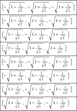
TraditionalForm[
  Column[ pts = {x, y, z} /.
          FullSimplify @ Solve[ D[h[x, y, z, λ1, λ2], #] == 0 & /@ {x, y, z, λ1, λ2},
                                      {x, y, z, λ1, λ2}], Frame -> All]]
A bit nicer way of finding all the solutions uses Grad - a new function in Mathematica 9 for vector analysis:
{x, y, z} /. Solve[ Grad[ h @@ #, #] == 0, #]& @ {x, y, z, λ1, λ2} // FullSimplify
The above table contains all critical points of the Lagrange function h. For sufficient conditions one can use Maximize and Minimize, e.g.:
FullSimplify @  ToRadicals @
Maximize[{f[x, y, z], g1[x, y] == 0, g2[x, z] == 0}, {x, y, z}]
{1 + Sqrt[2], {x -> -(1/Sqrt[2 + Sqrt[2]]),
               y -> -Sqrt[1 + 1/Sqrt[2]],
               z -> -Sqrt[1 + 1/Sqrt[2]]}}
We add a graphics with contours of constrained minima and maxima, the contraint functions ass well as all critical points of h:
Show[
  ContourPlot3D[{ f[x, y, z] ==  1 + Sqrt[2],
                  f[x, y, z] == -1 - Sqrt[2],
                  g1[x, y] == 0, g2[x, z] == 0},
                  {x, -2.3, 2.3}, {y, -2.3, 2.3}, {z, -2.3, 2.3},
                  ContourStyle -> {Directive[Cyan, Opacity[0.5]],
                                   Directive[Green, Opacity[0.5]],
                                   Directive[Orange, Opacity[0.15]],
                                   Directive[Orange, Opacity[0.15]]}, Mesh -> None],
  Graphics3D[{Magenta, PointSize[0.015], Point[pts]}]]

On the cyan surfaces we have maxima, on the green ones - minima and the solutions of the necessary conditions are denoted with the magenta points lying on the tube constraints.
Artes
- 57,212
- 12
- 157
- 245
12
Another possible way (using a hammer to kill a fly perhaps...) with the VariationalMethods package
<< VariationalMethods`

f[x_, y_, z_] := x y + y z
g1[x_, y_] := x^2 + y^2 - 2
g2[x_, z_] := x^2 + z^2 - 2

eqs =
 EulerEquations[
   f[x[t], y[t], z[t]] - (λ1[t] g1[x[t], y[t]] + λ2[t] g2[x[t], z[t]]),
   {x[t], y[t], z[t], λ1[t], λ2[t]}, t] /. x_[t] -> x;
See the resulting equations:
eqs//TableForm

(* y-2 x (λ1+λ2)==0
   x+z-2 y λ1==0
   y-2 z λ2==0
   2-x^2-y^2==0
   2-x^2-z^2==0 *)
And solve as the in the other answers!
{x,y,z}/.FullSimplify[Solve[eqs,{x,y,z,λ1,λ2}]]//TableForm
chuy
- 11,205
- 28
- 48
6
gradient[g_, vars_] :=  Table[D[g@@vars, vars[[j]]], {j, 1, Length[vars]}]

system1[lstConst_, vars_] := Join[ Join@@
Table[gradient[lstConst[[j]], vars], {j, 1, Length[lstConst]}],
Table[lstConst[[j]]@@vars,{j,1,Length[lstConst]}]];

system2[f_, lstConst_, vars_, lambda_] := Join[ gradient[f, vars] -
Sum[ lambda[[j]]*gradient[lstConst[[j]], vars], {j, 1,
Length[lstConst]}],Table[lstConst[[j]]@@vars, {j, 1, Length[lstConst]}]] ;

criticalPointsSystem1[lstConst_, vars_] :=   Solve[system1[lstConst, vars] ==
 Table[ 0, {j, 1, (Length[vars] + 1)*Length[lstConst]}],
vars] /. {(x_ -> y_) -> y} ;

criticalPointsSystem2[f_, lstConst_, vars_, lambda_] :=
Map[ Function [x, Take[x, Length[vars]]],
Solve[system2[f, lstConst, vars, lambda] ==
Table[0, {j, 1, Length[vars] + Length[lambda]}],
      Join[vars, lambda]]] /. {(x_ -> y_) -> y};

criticalPointsLagrangeM[f_, lstConst_, vars_, lambda_] :=
Join[criticalPointsSystem1[lstConst, vars],
criticalPointsSystem2[f, lstConst, vars, lambda]];


optimizeByLagrangeM[f_, lstConst_, vars_, lambda_, type_] :=
Which[ToUpperCase[type] == "MINIMIZE",Min[Map[Function[x, f @@ x],
criticalPointsLagrangeM[f, lstConst, vars, lambda]]],
ToUpperCase[type] == "MAXIMIZE", Max[Map[Function[x, f@@x],
criticalPointsLagrangeM[f, lstConst, vars, lambda]]],True,
Print["The given type of optimization problem is not supported"]];

f[x_, y_] := x; g[x_, y_] := y^2 + x^4 - x^3; (* test  *)

optimizeByLagrangeM[f, {g}, {x, y}, {\[Lambda]}, "MiNimize"]

optimizeByLagrangeM[f, {g}, {x, y}, {\[Lambda] }, "Maximize"]
TAWA
- 61
- 1
- 3
-
Hi ! Please, refer to the help centre and learn how to properly format your code and edit your post. – Sektor Mar 24 '15 at 19:25
-
-
Thank you ! Hope you stick around to contribute to the community :) ! + 1 BTW :D – Sektor Mar 24 '15 at 20:10
Minimize[{x y + y z, x^2 + y^2 - 2 == 0, x^2 + z^2 - 2 == 0}, {x, y}]and similarly withMaximize? Or do you insist on explicitly implementing the Lagrange method? – murray Jan 29 '14 at 14:53