How can I remove horizontal lines on a phase plot for a pendulum?

Question

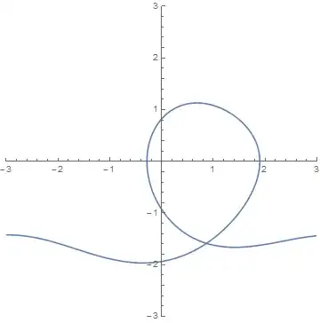
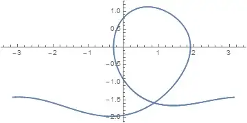
I am attempting to do a phase plot for a driven,damped pendulum. When the angle wraps from Pi to -Pi or -Pi to Pi I get a horizontal line on the plot. I would like to remove these lines as they mask the structure that is evident when plotting chaotic orbits. The function sss[t] performs the angle wrap and uses the piecewise function. Also I wanted to post the plot along with this question but could not find information on how to do it.

s = NDSolve[{\[Theta]''[t] + .5 \[Theta]'[t] + Sin[\[Theta][t]] == 
    1.35 Sin[2/3 t], \[Theta][0] == Pi/4, \[Theta]'[0] == 0}, {\[Theta],
    \[Theta]'}, {t, 0, 10000}];

 ss[t_] := Flatten[{\[Theta][t]} /. s]

 sss[t_] := Piecewise[{{Mod[ss[t][[1]], 2 Pi] - 2 Pi, 
            Mod[ss[t][[1]], 2 Pi] > Pi && ss[t][[1]] >= 0}, {Mod[ss[t][[1]], 
            2 Pi], Mod[ss[t][[1]], 2 Pi] < Pi && 
            ss[t][[1]] >= 0}, {-(Mod[-ss[t][[1]], 2 Pi] - 2 Pi), 
            Mod[-ss[t][[1]], 2 Pi] > Pi && 
            ss[t][[1]] < 0}, {-(Mod[-ss[t][[1]], 2 Pi]), 
            Mod[-ss[t][[1]], 2 Pi] < Pi && ss[t][[1]] < 0}, {ss[t][[1]], -Pi
            <= ss[t][[1]] <= Pi}}]

 ParametricPlot[Evaluate[{sss[t], \[Theta]'[t]} /. s], {t, 800, 1000}, 
 PlotRange -> 3]

Please learn how to upvote and downvote question and answers! — Dr. belisarius, Apr 02 '15 at 00:03
Welcome to Mathematica.SE! I suggest the following: 0) Browse the common pitfalls question 1) As you receive help, try to give it too, by answering questions in your area of expertise. 2) Read the [faq]! 3) When you see good questions and answers, vote them up by clicking the gray triangles, because the credibility of the system is based on the reputation gained by users sharing their knowledge. Also, please remember to accept the answer, if any, that solves your problem, by clicking the checkmark sign! — Dr. belisarius, Apr 02 '15 at 00:03
You need to use Exclusions with conditions on t. You need to find the values of t where the function is discontinuous. Using NDSolveValue should also simplify things. Don't return both theta and theta' from NDSolveValue. theta is sufficient, you can take the derivative later. See also if the third argument of Mod can simplify your Piecewise. — Szabolcs, Apr 02 '15 at 01:57
All of the answers below were extremely instructional. Many thanks! — Robert Martin, Apr 03 '15 at 13:57

Jens · Answer 1 · 2015-04-02T05:57:12.757

For a phase plot where one axis is an angle, you generally may not have a self-retracing curve, so you can't always count on being able to get a complete picture by just trimming the unnecessary repetitions of the curve - there may be no repetitions in $\theta'$ even if $\theta$ wraps around.

So here is a way to get the angle to fall within the fundamental interval $[-\pi, \,\pi]$ while not throwing away any part of the ParametricPlot:

s = First@
   NDSolve[{θ''[t] + .5 θ'[t] + Sin[θ[t]] == 
      1.35 Sin[2/3 t], θ[0] == Pi/4, θ'[0] == 
      0}, θ, {t, 0, 10000}];
plt = ParametricPlot[{θ[t], θ'[t]} /. s, {t, 800, 1000}];

remap[x_List] := Apply[{Mod[#1, 2 Pi, -Pi], #2} &, 
  SplitBy[x, Quotient[#[[1]], 2 Pi, Pi] &], {2}]

Show[plt /. Line[xx_] :> Line@remap[xx], 
 PlotRange -> {{-1.1 Pi, 1.1 Pi}, {-2, 2}}, Frame -> True]

wrapped

In plt, the ParametricPlot generates a single long line which contains the unwanted jumps. I use post-processing to get rid of those:

In plt, I find the contents of the Line, and modify them usingremap.

The function remap does the Mod operation with an offset specified in the third argument, as mentioned by Szabolcs in the comment. But before doing so, I use SplitBy to divide the content of the line according to the Quotient (the counterpart of Mod) of the $\theta$ entry divided by $2\pi$.

score 2 · Accepted Answer · answered Apr 02 '15 at 12:51

2

After some experimentation, I managed to use Exclusions to produce the following.

ParametricPlot[
  Evaluate[{sss[t], \[Theta]'[t]} /. s],
  {t, 799, 809},
  Exclusions -> {sss[t] == 0}
  ]

answered Apr 02 '15 at 12:51

TransferOrbit

3,547
13
26

This is how it should be done, but it's just unrealistically slow even with the radically reduced parameter range in your test. With the original range of t, I didn't have the patience to wait for a result... (+1) anyway. – Jens Apr 02 '15 at 15:40

score 1 · Answer 3 · answered Apr 02 '15 at 02:19

Undoubtedly, there are elegant ways to solve this problem. A quick and dirty approach is first to look at the line segments that make up the plot.

plt = ParametricPlot[Evaluate[{sss[t], \[Theta]'[t]} /. s], {t, 800, 1000}, 
 PlotRange -> 3];
Cases[plt, Line[{z__}] -> z, {0, Infinity}]

You will see that there are 3065 elements, enough to trace your curve many times over. Identify the beginning and end points of one cycle, here 4 ;; 149, and plot only that portion.

tem = Cases[plt, Line[{z__}] -> z, {0, Infinity}][[4 ;; 149]]; 
plt /. Line[{z__}] :> Line[tem]

Mathematica graphics

bbgodfrey · Answer 4 · 2015-04-02T15:49:11.780

Interestingly, although

r = First@NDSolve[{θ''[t] + .5 θ'[t] + Sin[θ[t]] == 1.35 Sin[2/3 t], 
    θ[0] == Pi/4, θ'[0] == 0}, θ, {t, 0, 10000}];
ParametricPlot[{Mod[θ[t], 2 Pi, -Pi], θ'[t]} /. r, {t, 980, 1000}, PlotRange -> All]

produces the undesired line,

Mathematica graphics

the simple change

s = θ /. r;
ParametricPlot[{Mod[s[t], 2 Pi, -Pi], s'[t]}, {t, 980, 1000}, PlotRange -> All]

does not.

Mathematica graphics

The more compact

s = NDSolveValue[{θ''[t] + .5 θ'[t] + Sin[θ[t]] == 1.35 Sin[2/3 t], 
    θ[0] == Pi/4, θ'[0] == 0}, θ, {t, 0, 10000}]
ParametricPlot[{Mod[s[t], 2 Pi, -Pi], s'[t]}, {t, 980, 1000}, PlotRange -> All]

also works well.

How can I remove horizontal lines on a phase plot for a pendulum?

4 Answers4

Linked