Best way to create symmetric matrices

Question

From time to time I need to generate symmetric matrices with relatively expensive cost of element evaluation. Most frequently these are Gram matrices where elements are $L_2$ dot products. Here are two ways of efficient implementation which come to mind: memoization and direct procedural generation.

ClearAll[el, elmem];
el[i_, j_] := Integrate[ChebyshevT[i, x] ChebyshevT[j, x], {x, -1, 1}];
elmem[i_, j_] := elmem[j, i] = el[i, j];

n = 30;
ClearSystemCache[];
a1 = Table[el[i, j], {i, n}, {j, n}]; // Timing
ClearSystemCache[];
a2 = Table[elmem[i, j], {i, n}, {j, n}]; // Timing
ClearSystemCache[];
(a3 = ConstantArray[0, {n, n}];
  Do[a3[[i, j]] = a3[[j, i]] = el[i, j], {i, n}, {j, i}];) // Timing
a1 == a2 == a3

---

{34.75, Null}

{18.235, Null}

{18.172, Null}

True

Here a1 is a redundant version for comparison, a2 is using memoization, a3 is a procedural-style one which I don't really like but it beats the built-in function here. The results are quite good but I wonder if there are more elegant ways of generating symmetric matrices?

---

SUMMARY (UPDATED)

Thanks to all participants for their contributions. Now it's time to benchmark. Here is the compilation of all proposed methods with minor modifications.

array[n_, f_] := Array[f, {n, n}];
arraymem[n_, f_] := 
  Block[{mem}, mem[i_, j_] := mem[j, j] = f[i, j]; Array[mem, {n, n}]];
proc[n_, f_] := Block[{res},
  res = ConstantArray[0, {n, n}]; 
  Do[res[[i, j]] = res[[j, i]] = f[i, j], {i, n}, {j, i}];
  res
  ]

acl[size_, fn_] := 
  Module[{rtmp}, rtmp = Table[fn[i, j], {i, 1, size}, {j, 1, i}];
   MapThread[Join, {rtmp, Rest /@ Flatten[rtmp, {{2}, {1}}]}]];

RM1[n_, f_] := 
  SparseArray[{{i_, j_} :> f[i, j] /; i >= j, {i_, j_} :> f[j, i]}, n];
RM2[n_, f_] := 
  Table[{{i, j} -> #, {j, i} -> #} &@f[i, j], {i, n}, {j, i}] // 
    Flatten // SparseArray;

MrWizard1[n_, f_] := 
  Join[#, Rest /@ #~Flatten~{2}, 2] &@Table[i~f~j, {i, n}, {j, i}];
MrWizard2[n_, f_] := Max@##~f~Min@## &~Array~{n, n};

MrWizard3[n_, f_] := Block[{f1, f2},
  f1 = LowerTriangularize[#, -1] + Transpose@LowerTriangularize[#] &@
     ConstantArray[Range@#, #] &;
  f2 = {#, Reverse[(Length@# + 1) - #, {1, 2}]} &;
  f @@ f2@f1@n
  ]


whuber[n_Integer, f_] /; n >= 1 := 
  Module[{data, m, indexes}, 
   data = Flatten[Table[f[i, j], {i, n}, {j, i, n}], 1];
   m = Binomial[n + 1, 2] + 1;
   indexes = 
    Table[m + Abs[j - i] - Binomial[n + 2 - Min[i, j], 2], {i, n}, {j,
       n}];
   Part[data, #] & /@ indexes];

JM[n_Integer, f_, ori_Integer: 1] := 
  Module[{tri = Table[f[i, j], {i, ori, n + ori - 1}, {j, ori, i}]}, 
   Fold[ArrayFlatten[{{#1, Transpose[{Most[#2]}]}, {{Most[#2]}, 
        Last[#2]}}] &, {First[tri]}, Rest[tri]]];

generators = {array, arraymem, proc, acl, RM1, RM2, MrWizard1, 
   MrWizard2, MrWizard3, whuber, JM};

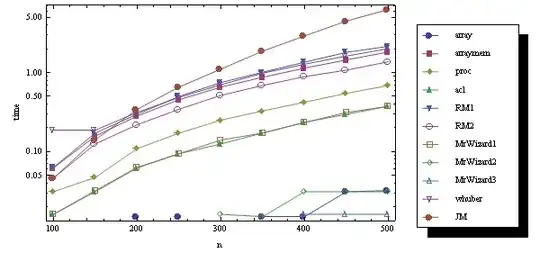
The first three procedures are mine, all other are named after their authors. Let's start from cheap f and (relatively) large dimensions.

fun = Cos[#1 #2] &;
ns = Range[100, 500, 50]
data = Table[ClearSystemCache[]; Timing[gen[n, fun]] // First,
   {n, ns}, {gen, generators}];

Here is a logarithmic diagram for this test:

<< PlotLegends`

ListLogPlot[data // Transpose, PlotRange -> All, Joined -> True, 
 PlotMarkers -> {Automatic, Medium}, DataRange -> {Min@ns, Max@ns}, 
 PlotLegend -> generators, LegendPosition -> {1, -0.5}, 
 LegendSize -> {.5, 1}, ImageSize -> 600, Ticks -> {ns, Automatic}, 
 Frame -> True, FrameLabel -> {"n", "time"}]

Now let's make f numeric:

fun = Cos[N@#1 #2] &;

The result is quite surprising:

As you may guess, the missed quantities are machine zeroes.

The last experiment is old: it doesn't include fresh MrWizard3 and RM's codes are with //Normal. It takes "expensive" f from above and tolerant n:

fun = Integrate[ChebyshevT[#1 , x] ChebyshevT[#2, x], {x, -1, 1}] &;
ns = Range[10, 30, 5]

The result is

As we see, all methods which do not recompute the elements twice behave identically.

Answer 1

Proposed solution

If fn[i,j] produces the $(i,j)^{th}$ element, then

makeSym[size_, fn_] := Module[
  {rtmp},
  rtmp = Table[
    fn[i, j],
    {i, 1, size},
    {j, 1, i}];
  MapThread[
   Join,
   {rtmp, Rest /@ Flatten[rtmp, {{2}, {1}}]}
   ]
  ]

does what you want.

Example

makeSym[5, Subscript[f, #1, #2] &] // MatrixForm

How does it work?

Idea

Produce half the matrix, then do a "ragged transpose" and finally zip the results together.

Step by step

First, we construct half the matrix with a Table: For an example size of 5, we have

With[{size = 5},rtmp=Table[fn[i, j], {i, 1, size}, {j, 1, i}]]

(*
{ {fn[1, 1]}, 
  {fn[2, 1], fn[2, 2]}, 
  {fn[3, 1], fn[3, 2], fn[3, 3]}, 
  {fn[4, 1], fn[4, 2], fn[4, 3], fn[4, 4]}, 
  {fn[5, 1], fn[5, 2], fn[5, 3], fn[5, 4], fn[5, 5]}}
*)

Next, use the form of Flatten described here and in the docs to do a "ragged transpose":

Flatten[rtmp, {{2}, {1}}]
(*
{ {fn[1, 1], fn[2, 1], fn[3, 1], fn[4, 1], fn[5, 1]}, 
  {fn[2, 2], fn[3, 2], fn[4, 2], fn[5, 2]}, 
  {fn[3, 3], fn[4, 3], fn[5, 3]}, 
  {fn[4, 4], fn[5, 4]}, 
  {fn[5, 5]}}
*)

then drop the first element of each (to avoid duplicating it), by mapping Rest:

Rest /@ Flatten[rtmp, {{2}, {1}}]

(*
{ {fn[2, 1], fn[3, 1], fn[4, 1], fn[5, 1]}, 
  {fn[3, 2], fn[4, 2], fn[5, 2]}, 
  {fn[4, 3], fn[5, 3]}, 
  {fn[5, 4]}, 
  {}}
*)

And finally, zip together the corresponding pieces (ie, the $i^{th}$ line of the last result with the $i^{th}$ of rtmp), using MapThread:

MapThread[
 Join,
 {rtmp, Rest /@ Flatten[rtmp, {{2}, {1}}]}
 ]

(*
{ {fn[1, 1], fn[2, 1], fn[3, 1], fn[4, 1], fn[5, 1]}, 
  {fn[2, 1], fn[2, 2], fn[3, 2], fn[4, 2], fn[5, 2]}, 
  {fn[3, 1], fn[3, 2], fn[3, 3], fn[4, 3], fn[5, 3]}, 
  {fn[4, 1], fn[4, 2], fn[4, 3], fn[4, 4], fn[5, 4]}, 
  {fn[5, 1], fn[5, 2], fn[5, 3], fn[5, 4], fn[5, 5]}}
*)

Answer 2

Borrowing liberally from acl's answer:

sim = Join[#, Rest /@ # ~Flatten~ {2}, 2] & @ Table[i ~#~ j, {i, #2}, {j, i}] &;

sim[Subscript[x, ##] &, 5] // Grid

$\begin{array}{ccccc} x_{1,1} & x_{2,1} & x_{3,1} & x_{4,1} & x_{5,1} \\ x_{2,1} & x_{2,2} & x_{3,2} & x_{4,2} & x_{5,2} \\ x_{3,1} & x_{3,2} & x_{3,3} & x_{4,3} & x_{5,3} \\ x_{4,1} & x_{4,2} & x_{4,3} & x_{4,4} & x_{5,4} \\ x_{5,1} & x_{5,2} & x_{5,3} & x_{5,4} & x_{5,5} \end{array}$

Trading efficiency for brevity:

sim2[f_, n_] := Max@## ~f~ Min@## & ~Array~ {n, n}

sim2[Subscript[f, ##] &, 5] // Grid

$\begin{array}{ccccc} x_{1,1} & x_{2,1} & x_{3,1} & x_{4,1} & x_{5,1} \\ x_{2,1} & x_{2,2} & x_{3,2} & x_{4,2} & x_{5,2} \\ x_{3,1} & x_{3,2} & x_{3,3} & x_{4,3} & x_{5,3} \\ x_{4,1} & x_{4,2} & x_{4,3} & x_{4,4} & x_{5,4} \\ x_{5,1} & x_{5,2} & x_{5,3} & x_{5,4} & x_{5,5} \end{array}$

---

Just for fun, here's a method for fast vectorized (Listable) functions such as your "cheap f" test, showing what's possible if you keep everything packed. (Cos function given a numeric argument so that it evaluates.)

f1 = LowerTriangularize[#, -1] + Transpose@LowerTriangularize[#] & @
       ConstantArray[Range@#, #] &;

f2 = {#, Reverse[(Length@# + 1) - #, {1, 2}]} &;

f3 = # @@ f2@f1 @ #2 &;

f3[Cos[N@# * #2] &, 500]  // timeAvg

sim[Cos[N@# * #2] &, 500] // timeAvg

0.00712

0.1436

Answer 3

A simple and clean way to generate symmetric matrices (in general) would be the following:

SparseArray[{{i_, j_} :> f[i, j] /; i >= j, {i_, j_} :> f[j, i]}, 5] // Normal

(* {{f[1, 1], f[2, 1], f[3, 1], f[4, 1], f[5, 1]}, 
    {f[2, 1], f[2, 2], f[3, 2], f[4, 2], f[5, 2]}, 
    {f[3, 1], f[3, 2], f[3, 3], f[4, 3], f[5, 3]}, 
    {f[4, 1], f[4, 2], f[4, 3], f[4, 4], f[5, 4]}, 
    {f[5, 1], f[5, 2], f[5, 3], f[5, 4], f[5, 5]}} *)

The Normal is necessary only if you don't want a SparseArray object (generally, it doesn't matter). If your function f is expensive, you can do something like

Table[{{i, j} -> #, {j, i} -> #} &@f[i, j], {i, 5}, {j, i}] // Flatten // SparseArray

which evaluates f only $N(N+1)/2$ times instead of $N^2$.

Answer 4

I might as well. Here's my variation, which uses a "bordering" method to build up a symmetric matrix from a triangular array:

tri = Table[C[i, j], {i, 5}, {j, i}];

Fold[ArrayFlatten[{{#1, Transpose[{Most[#2]}]}, {{Most[#2]}, Last[#2]}}] &,
     {First[tri]}, Rest[tri]]

{{C[1, 1], C[2, 1], C[3, 1], C[4, 1], C[5, 1]},
 {C[2, 1], C[2, 2], C[3, 2], C[4, 2], C[5, 2]},
 {C[3, 1], C[3, 2], C[3, 3], C[4, 3], C[5, 3]},
 {C[4, 1], C[4, 2], C[4, 3], C[4, 4], C[5, 4]},
 {C[5, 1], C[5, 2], C[5, 3], C[5, 4], C[5, 5]}}

Here's a demonstration of why the method is called "bordering":

Here's a function that acts like Array[]:

SymmetricArray[f_, n_Integer, ori_Integer: 1] := 
 Module[{tri = Table[f[i, j], {i, ori, n + ori - 1}, {j, ori, i}]}, 
        Fold[ArrayFlatten[{{#1, Transpose[{Most[#2]}]}, {{Most[#2]}, Last[#2]}}] &,
             {First[tri]}, Rest[tri]]]

Try it out:

SymmetricArray[Min, 5]
{{1, 1, 1, 1, 1}, {1, 2, 2, 2, 2}, {1, 2, 3, 3, 3}, {1, 2, 3, 4, 4}, {1, 2, 3, 4, 5}}

Answer 5

What about

Table[x[Max[i, j], Min[i, j]], {i, 1, 6}, {j, 1, 6}] // MatrixForm

Answer 6

Commenters have pointed out there is no timing gain. But, in the hopes of stimulating better answers from others, here's a start.

SymmetricTable[f_, n_Integer] /; n >= 1 := Module[{data, m, indexes},
   data = Flatten[Table[f[i, j], {i, n}, {j, i, n}], 1];
   m = Binomial[n + 1, 2] + 1;
   indexes = Table[m + Abs[j - i] - Binomial[n + 2 - Min[i, j], 2], {i, n}, {j, n}];
   Part[data, #] & /@ indexes
   ];

It tabulates the upper triangle of f, flattens it into a vector (data), computes a symmetric array of subscripts into that vector (indexes), and applies those subscripts to the vector to obtain the symmetrized square table. Whether that is "elegant" or not will be somewhat subjective.

As an example of usage:

f = Function[{i, j}, Sow[{i, j}];  10 i + j];
Reap[SymmetricTable[f, 5] // MatrixForm]

This returns a symmetric table of values of f along with a list of the arguments that were passed to f when constructing this table, verifying that the minimum number of calls to f were actually made.