The reason why you get a factor of 500 of I have explained in my comment. Let's replace your g with a better behaved function:
mass = 100;
width = 10^-2;
g[x_] := mass/width HeavisideLambda[x/width]
This is a triangular peak with area 100 and basewidth 0.01.
Now let's impose the desired boundary conditions of $\partial u / \partial x =0$ at the boundaries:
Derivative[1, 0][u][-10, t] == 0
Derivative[1, 0][u][10, t] == 0
Now back to your code:
pde = D[u[x, t], t] - 0.2 D[D[u[x, t], {x, 1}], {x, 1}] == 0;
sol = NDSolve[{pde, u[x, 0] == g[x], Derivative[1, 0][u][-10, t] == 0,
   Derivative[1, 0][u][10, t] == 0}, u[x, t], {x, -10, 10}, {t, 0, 20}]
This will of course complain due to the absence of a continuous derivative (much less, a continuous second derivative) of g[x], but it will come up with something.
Plot3D[u[x, t] /. sol, {x, -5, 5}, {t, 0, 20}, PlotRange -> Full]

Huge peak at the beginning (just a finite approximation of a delta-function).
Plot3D[u[x, t] /. sol, {x, -10, 10}, {t, 0, 20}]

Something saner, as diffusion takes place.
{-10, 10} is quite a large box. It's hard to see, that the process of diffusion is really contained within it. Let's confine the region a bit and give more time to develop.
sol = NDSolve[{pde, u[x, 0] == g[x], Derivative[1, 0][u][-3, t] == 0,
    Derivative[1, 0][u][3, t] == 0}, u[x, t], {x, -3, 3}, {t, 0, 50}]
Plot3D[u[x, t] /. sol, {x, -3, 3}, {t, 0, 30}, PlotRange -> {0, 30}]
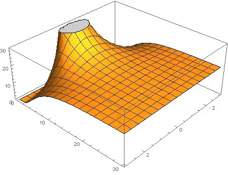
Now the peak fills the box up to about 15.
NIntegrate[u[x, t] /. (First@sol) /. t -> 0, {x, -0.1, 0.1}]
100.08
I've chosen this range, because at t=0 the peak is a bit narrow and NIntegrate can miss it.
Let's check, how everything evolves with time:
Do[Print[NIntegrate[u[x, t] /. (First@sol) /. t -> tt, {x, -3, 3}]],
   {tt, {1, 5, 10, 20, 30, 40}}]
100.08
100.08
100.08
100.08
100.08
100.08
Very consistent. But I don't like the 0.08 error. Let's try to make NDSolve's job a bit easier by specifying easier initial conditions (broader peak, so numerical precision isn't so much of an issue).
mass = 100;
width = 1;
g[x_] := mass /width HeavisideLambda[x/width]
sol = NDSolve[{pde, u[x, 0] == g[x], Derivative[1, 0][u][-3, t] == 0,
   Derivative[1, 0][u][3, t] == 0}, u[x, t], {x, -3, 3}, {t, 0, 50}]
Do[Print[NIntegrate[u[x, t] /. (First@sol) /. t -> tt, {x, -3, 3}]],
   {tt, {1, 5, 10, 20, 30, 40}}]
100.
100.
100.
100.
100.
100.
EDIT follow-up for ill-defined peak functions :-)
Clear[g]; deltaPos = 0;
g[x_] := Piecewise[{{0, x < deltaPos}, {100, x == deltaPos}, {0, x > deltaPos}}]
pde = D[u[x, t], t] - 0.2 D[D[u[x, t], {x, 1}], {x, 1}] == 0;
sol = NDSolve[{pde, u[x, 0] == g[x], Derivative[1, 0][u][-10, t] == 0,
    Derivative[1, 0][u][10, t] == 0}, u[x, t], {x, -10, 10}, {t, 0, 50}]
Plot3D[u[x, t] /. sol, {x, -3, 3}, {t, 0.1, 3}, PlotRange -> Full]
produces this (below), as x=0 is included in the initial sampling points.

Naturally, NDSolve complains about reaching the maximum of allowed grid points, because it detects a peak in g[x], but can't get a handle on how narrow it is:
NDSolve::mxsst: Using maximum number of grid points 10000 allowed by the MaxPoints or MinStepSize options for independent variable x.
Clear[g]; deltaPos = 2;
g[x_] := Piecewise[{{0, x < deltaPos}, {100, x == deltaPos}, {0, x > deltaPos}}]
With a definition like above NDSolve shuts up and returns u[x, t] that is zero across the domain. The initial sampling grid seems to be rather coarse. It simply doesn't realize, that there's an out-of-place peak in your starting function. deltaPos = 5 is, however, among the sampling points. That returns a much saner result, similar to what we get for deltaPos = 0. The lesson to learn is "define your point sources properly".
Thanks for asking the question, it brought a great deal about solving ODEs with Mathematica to my attention, especially in the linked question in the comments.
InitCompparameter is never used. The factor 500 is 100/0.2. – b.gates.you.know.what Apr 29 '15 at 11:49x=-10andx=10are completely invalid. A peculiarity of the diffusion equation is that perturbations propagate instantaneously. Another thing is the way, your "delta-function" is defined.NDSolvegives an message that it is looking at 10000 grid points for x. The interval for x is{-10,10}thus it might mistakenly interpret the single point ofg[x]=100as a peak of width around 0.002 and height up to 100 giving a total mass of around 0.2 (500 smaller than the desired 100. If I increase the x range to{-20,20}the solution becomes twice as large. – LLlAMnYP Apr 29 '15 at 15:02