How to draw a cobweb graph like this one?

Question

How to draw a cobweb graph like this one with tikz?

Reading other topics, this is what i got so far:

\documentclass{article}
\usepackage{tikz}
\usetikzlibrary{arrows}
\begin{document}
\begin{figure}[htbp]
\centering
\newcounter{j}
\begin{tikzpicture}[>=latex',scale=10,
     declare function={%
         p(\t)=  greater(\t,0.5)  ? 1 :  2* \t ;}]

    \draw[color=blue,domain=-0:1.05] plot (\x,{\x^3});

    \drawcolor=green--(1.1,1.1);
    \draw->--(0,1) node[above]{$y$};
    \draw->--(1,0) node[right]{$x$};
    \newcommand{\x}{.1}
    \foreach \i in {1,...,4}{%
       \pgfmathparse{(p(\x)}
       \let\y\pgfmathresult
       \drawcolor=magenta--(\x,\y)--(\y,\y);
       \draw[color=orange,dotted,line width=0.8pt]%
            (\x,\x)--(\x,0) node[below=8pt]{$u_\i$};
       \pgfmathsetcounter{j}{\i+1}
       \draw[color=blue,dotted,line width=0.8pt]%
            (\x,\y)--(0,\y) node[left=8pt] {$u_\thej$};
       \global\let\x\y}

\end{tikzpicture}
\end{figure}
\end{document}

Answer 1

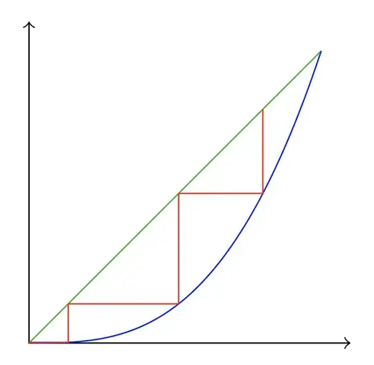
Here is an outline to get you started. The idea is to define (declare) a function f(\x). After the function and line are plotted, we use \foreach to perform a set number of iterations. Use \evaluate in the for loop to calculate \newv, the value of the function at the start value \startv. Then draw vertically to the function and horizontally to the line using \draw (\startv,\startv)|-(\newv,\newv);. Finally reset the value of \startv to the calculated value \newv and loop.

The code is

\documentclass{article}
\usepackage{tikz}
\newcommand{\startv}{.8}
\begin{document}
\begin{tikzpicture}[scale=3,declare function={f(\x)=\x\x\x;}]
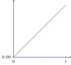
\draw<->|-(1.1,0);
\draw[green!70!black] (0,0)--(1,1);
\draw[blue, domain=0:1, smooth] plot (\x,{f(\x)});
\foreach \t[evaluate=\t as \newv using f(\startv)] in {1,...,4}{
    \draw[red] (\startv,\startv)|-(\newv,\newv);
    \xdef\startv{\newv}}
\end{tikzpicture}
\end{document}

You can easily change the function, start value, and number of iterations.

For example: Set f(\x)=3.2*\x*(1-\x);. Change \newcommand{\startv}{.25}, and loop 100 times with {1,...,100} to produce the image

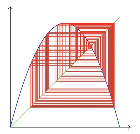
Similarly, f(\x)=3.8*\x*(1-\x); gives us

You could put the whole thing into a macro called \cobweb with three arguments (one optional):

\cobweb[<start value>]{<function>}{<iterations>}

<start value> is optional (default=.5), <function> must use \x for the variable. Sample use:

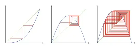
\cobweb[.8]{\x*\x*\x}{4}\qquad
\cobweb[.25]{3.2*\x*(1-\x)}{100}\qquad
\cobweb{3.8*\x*(1-\x)}{100} 

produces

Here is the code with the macro:

\documentclass{article}
\usepackage{tikz}
\newcommand{\cobweb}[3][.5]{% \cobweb[<start value>]{<function>}{<iterations>}
    \begin{tikzpicture}[scale=3,declare function={f(\x)=#2;}]
    \xdef\startv{#1}
    \draw<->|-(1.1,0);
    \draw[green!70!black] (0,0)--(1,1);
    \draw[blue, domain=0:1, smooth] plot (\x,{f(\x)});
    \foreach \t[evaluate=\t as \newv using f(\startv)] in {1,...,#3}{
    \draw[red] (\startv,\startv)|-(\newv,\newv);
    \xdef\startv{\newv}}
    \end{tikzpicture}}
\begin{document}
\cobweb[.8]{\x\x\x}{4}\qquad
\cobweb[.25]{3.2\x(1-\x)}{100}\qquad
\cobweb{3.8\x(1-\x)}{100}
\end{document}

Update:

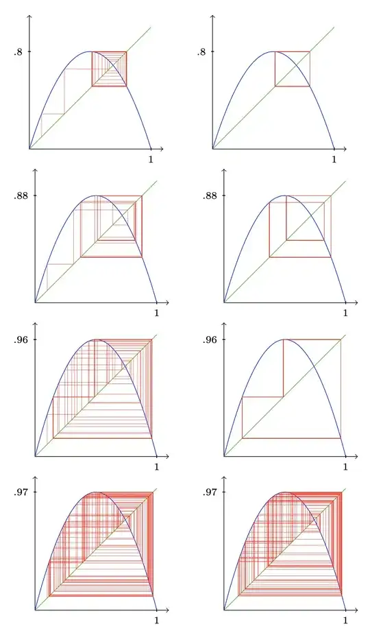
I decided to keep playing with this to examine the bifurcating and chaotic behavior found by iterating the family of functions f(x)=4λx(1-x). That function is now built in to a macro \bifur that takes 4 arguments, one optional:

\bifur[<skip>]{<start value>}{<lambda>}{<iterations>}

The optional argument <skip> will not plot the first <skip> iterations of the function to see the long-term behavior. If omitted, no iterations will be skipped. For example, to skip the first 50 iterations and draw the next 100 (and compare with skip=0):

\bifur{.1}{.8}{100}\qquad
\bifur[50]{.1}{.8}{100}
\bifur{.1}{.88}{100}\qquad
\bifur[50]{.1}{.88}{100}
\bifur{.1}{.96}{100}\qquad
\bifur[50]{.1}{.96}{100}
\bifur{.1}{.97}{100}\qquad
\bifur[50]{.1}{.97}{100}

Here is the code with the \bifur macro:

\documentclass{article}
\usepackage{tikz,ifthen}
\tikzset{tick/.style={draw, minimum width=0pt, minimum height=2pt, inner sep=0pt, label=below:$\scriptstyle#1$},
    tick/.default={}}
\newcommand{\bifur}[4][0]{% \bifur[<skip>]{<start value>}{<lambda>}{<iterations>}
    \begin{tikzpicture}[scale=3,declare function={f(\x)=#34\x*(1-\x);}]
    \draw<->|-(1.1,0);
    \node[tick=1] at (1,0){}; \node[tick=#3,rotate=-90] at (0,#3){};
    \xdef\startv{#2}
    \draw[green!70!black] (0,0)--(1,1);
    \draw[blue, domain=0:1, smooth] plot (\x,{f(\x)});
    \ifthenelse{#1=0}{}{
    \foreach \t[evaluate=\t as \newv using f(\startv)] in {1,...,#1}{
    \xdef\startv{\newv}}}
    \foreach \t[evaluate=\t as \newv using f(\startv)] in {1,...,#4}{
    \draw[red, very thin, line cap=round, line join=round] (\startv,\startv)|-(\newv,\newv);
    \xdef\startv{\newv}}
    \end{tikzpicture}}
\begin{document}
\bifur{.1}{.8}{100}\qquad
\bifur[50]{.1}{.8}{100}
\end{document}

Here is is turned into a gif:

Answer 2

I translate TikZ code of @Sandy G to Asymptote.

// COBWEB
// Run on http://asymptote.ualberta.ca/
// Asymptote translation from Sandy G at
// https://tex.stackexchange.com/a/640044/140722
unitsize(5cm);
import graph;
real f(real x){return 3.8*x*(1-x);}
path gf=graph(f,0,1);
draw((1.1,0)--(0,0)--(0,1.1),Arrows(TeXHead));
draw((0,0)--(1,1),.7green);
draw(gf,blue);
real startv=.5;
int n=50;
for(int i=1; i<n; ++i){
real newv=f(startv);
draw((startv,startv)--(startv,newv)--(newv,newv),red);

startv=newv;
}
shipout(bbox(5mm,invisible));