Is there an easy way to plot Jacobi Elliptic Functions with Tikz-PGF?

Question

So The Jacobi Elliptic Functions are a little bit tricky to plot because they depend on the complete elliptic integral of the first kind K(k) that can be written as a sum of double factorials, and the Fourier series for the Jacobi Elliptic Functions then depend on exponentials of these elliptic integrals, I can easily write all the mathematical formulas, but I don't know an easy way to represent them on Tikz or PGF, probably gnuplot would be the easiest but I would like to make it depend only on Tikz PGF because of configurations problems I am having with gnuplot, and I would like to write that in a formulaic form, instead of a table because I would like to change a parameter easily from one compilation to another.

Basically, is there a way to calculate summations and double factorials in Tikz - PGF on some variables and then use them in a plot of a function that will depend on those ?

Bassically I need a way of calculating:

K(k) = pi/2 sum[n=0:10] ((( 2 * n - 1)!!)/((2 * n)!!)) * (k^(2*n)) 

and for a given u and v= sqrt(1-u^2)

q = exp(-pi * (K(v)/K(u))) 

calculate and plot for example:

sn_u(x) = (2* pi/(K(u) * u)) * sum[n=0:5] (((q^(n+0.5)) * sin((2*n+1) * x * pi/(2 * K(u))))/(1-(q^(2n+1))))

How do I implement these sums and double factorial as a function? Also is there a way to make these calculations modular in the way I wrote them?

Answer 1

I can't tell more because my mathematical ability is limited.

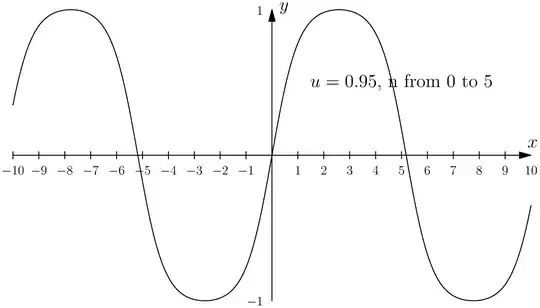
The following incompleted code, in Asymptote, can be compiled on http://asymptote.ualberta.ca/.

import graph;
import gsl; // https://github.com/vectorgraphics/asymptote/blob/master/gsl.cc
// 1086 addGSLDOUBLEFunc<gsl_sf_ellint_Kcomp>(SYM(K),SYM(k));
// in asy code, it is 'real K(real k)'
// for gsl_sf_ellint_Kcomp, see 
// https://www.gnu.org/software/gsl/doc/html/specfunc.html?highlight=bessel#c.gsl_sf_ellint_Kcomp and 
// https://www.gnu.org/software/gsl/doc/html/specfunc.html?highlight=gsl_prec_double#c.gsl_mode_t.GSL_PREC_DOUBLE
size(350,200,false);
real q(real k){ return exp(-pi*(K(sqrt(1-k^2))/K(k)));}
typedef real newreal(real);
// Define the function "sn_u(real k, int n)"
newreal sn_u(real k, int n){
  return new real(real x)
  {
    real createfunction(int n)
    {
      return ((q(k)^(n+0.5)) * sin((2n+1)  x * pi/(2 * K(k))))/(1-(q(k)^(2n+1)));
    }
    return (2pi)/(K(k)k)*sum(sequence(createfunction,n));
  // See T[] sequence(T f(int), int n) and T sum(T[] a)
  // in 6.12 Arrays of the documentation.
  };
}
// the graph
guide g=graph(sn_u(0.95,6),-10,10,350);
draw(g);
label("$u=0.95$, n from 0 to 5",(5,0.5));
// for axes
xaxis(Label("$x$",position = EndPoint, align=NE),
      xmin=-10,
      Ticks(scale(.7)*Label(),
            NoZero, end=false, Step=1, Size=.8mm, size=.4mm,
            pTick=black),
            Arrow);
yaxis(Label("$y$",position = EndPoint, align=NE),
      ymin=-1,ymax=1,
      Ticks(scale(.7)*Label(),
            NoZero, begin=false, end=false, Step=1, Size=.8mm, size=.4mm,
            pTick=black),
      Arrow);

Answer 2

Here is my solution, a bit late.

\documentclass{standalone}
\usepackage{pgfplots}
\pgfplotsset{compat=1.15}
\begin{document}
     \begin{tikzpicture}[
     declare function={
        K(\u) = pi/2*(1+(\u^2)/4+9*(\u^4)/64+25*(\u^6)/(16*16));
        I(\x,\i)=((e^(-(\i+0.5)*pi*K(0.3)/K(0.95)))*sin(deg((2*\i+1)*\x*pi/(2*K(0.95)))))/(1-(e^(-(2*\i+1)*pi*K(0.3)/K(0.95))));
        sn(\x)=2*pi/(0.95*K(0.95))*(I(\x,0)+I(\x,1)+I(\x,2)+I(\x,3)+I(\x,4)+I(\x,5));
    }
    ]
    \begin{axis}[
        axis lines = middle,
        axis equal image,
        xlabel = $x$,
        ylabel = {$y$},
        domain=-5:5,
        ymax=2,ymin=-2,
        samples=100,
        grid=major,
        ]
        \addplot [color=blue] {sn(x)};
    \end{axis}
\end{tikzpicture}
\end{document}