How to plot a system of equations in Latex Pgfplots?

Question

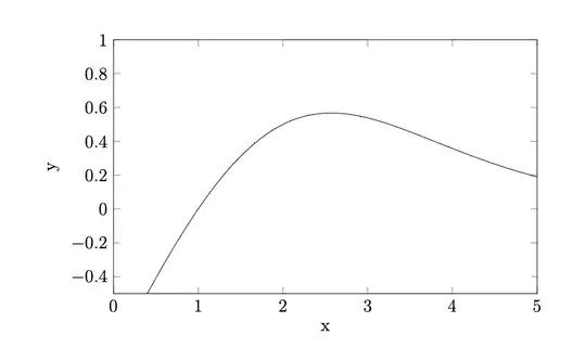
I plotted a function in Latex that worked very well:

\begin{figure}[htbp!]
  \centering
  \begin{tikzpicture}
     \begin{axis}[
      legend pos=north east,
      title = {},
      xlabel = {x},
      ylabel = {y},
      xmin = 0, xmax = 5,
      ymin = -0.5, ymax = 1,
      xtick = {0, 1, 2, 3, 4, 5},
      ytick = {-0.4, -0.2, 0.0, 0.2, 0.4, 0.6, 0.8, 1.0},
      height=6cm,
      width=10cm
      ]
      \addplot[black, no marks, domain=0.0:5, smooth]
      {(x-1)*(exp(-x+2)/(1+exp(-x+2)))};
    \end{axis}
  \end{tikzpicture}
\end{figure}

which generates:

But now I have to plot a system of equations:

Any ideas on how to plot system of equations in Latex PgfPlots?

Thank you very much!

Welcome to TeX.SX! It is always better to post a minimal working example (MWE). You can solve this problem by making two plots (with \addplot) for the two cases with different settings for domain=.... — dexteritas, Sep 08 '22 at 14:18

score 1 · Answer 1 · answered Sep 08 '22 at 15:29

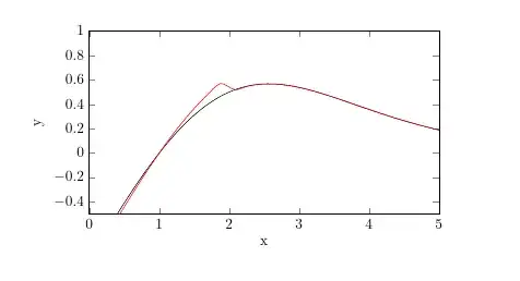
As a possible different approach, especially useful if complexity go up, consider that pgfmath has the ternary operator (x<a ? case true : case false) and that you can quite naturally define functions in one site and use them.

\documentclass{article}
\usepackage{pgfplots}\pgfplotsset{compat=1.18}
\begin{document}
\tikzset{declare function={
        s(\x)=exp(-\x+2)/(1+exp(-\x+2));
        f(\x)=(\x<2)?((\x-1)s(\x-0.5)):((\x-1)s(\x));
}}
\begin{tikzpicture}
     \begin{axis}[
      legend pos=north east,
      title = {},
      xlabel = {x},
      ylabel = {y},
      xmin = 0, xmax = 5,
      ymin = -0.5, ymax = 1,
      xtick = {0, 1, 2, 3, 4, 5},
      ytick = {-0.4, -0.2, 0.0, 0.2, 0.4, 0.6, 0.8, 1.0},
      height=6cm,
      width=10cm
      ]
      \addplot[black, no marks, domain=0.0:5, smooth] {(x-1)*s(x)};
      \addplot[red, no marks, domain=0.0:5, smooth] {(f(x)};
    \end{axis}
  \end{tikzpicture}
\end{document}

That method has its own challenges. Your plot is not right. Try to add \addplot[green, no marks, domain=0.0:5, samples=1000] {(f(x)}; — hpekristiansen, Oct 08 '22 at 19:14

score 0 · Answer 2 · answered Sep 08 '22 at 14:28

I found the answer, maybe it'll helpful for someone:

\usepackage{pgfplots}
\pgfplotsset{width=10cm,compat=newest}
\begin{document}
\begin{figure}[htbp!]
  \centering
  \begin{tikzpicture}
     \begin{axis}[
      legend pos=north east,
      title = {},
      xlabel = {x},
      ylabel = {y},
      xmin = 0, xmax = 5,
      ymin = -0.5, ymax = 1,
      xtick = {0, 1, 2, 3, 4, 5},
      ytick = {-0.4, -0.2, 0.0, 0.2, 0.4, 0.6, 0.8, 1.0},
      height=6cm,
      width=10cm
      ]
\plot[black, no marks, domain=0:2, smooth]
  function{(x-1)*(exp(-(x-0.5)+2)/(1+exp(-(x-0.5)+2)))};
\plot[black, no marks, domain=2:5, smooth]
  function{(x-1)*(exp(-x+2)/(1+exp(-x+2)))};
\end{axis}

\end{tikzpicture}
\end{figure}
\end{document}

Any particular reason for switching from the pgfplots syntax \addplot [...] {<function>}; to the TikZ syntax \plot [...] function {<function>};? — Torbjørn T., Sep 08 '22 at 15:10

score 0 · Answer 3 · answered Oct 09 '22 at 03:54

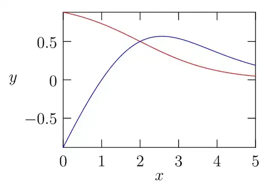
Asymptote for comparison, also see this. asy code can be embbed into .tex document.

// http://asymptote.ualberta.ca/
unitsize(1cm,2cm);
import graph;
real s(real x){return exp(2-x)/(1+exp(2-x));}
real f(real x){
if (x<-2) 
  return (x-1)*s(x-.5);
else  
  return (x-1)*s(x);
}
path gs=graph(s,0,5);
path gf=graph(f,0,5);
draw(gs,red);
draw(gf,blue);
xaxis("$x$",BottomTop,LeftTicks(Step=1));
yaxis("$y$",LeftRight,RightTicks(Step=.5));
shipout(bbox(5mm,invisible));

How to plot a system of equations in Latex Pgfplots?

3 Answers3