1

I'm trying to produce something like the figure below but in 3D so that I can plot discrete point mass functions. The only example I could find in the pgfplots manual is on page 111, but I couldn't figure out how to modify it to my needs – I think it's the wrong starting place anyway.

I created this figure using simple draw commands:

enter image description here

Qrrbrbirlbel
  • 119,821
TonyK
  • 625
  • 2
  • 9

2 Answers2

1

In my opinion, if one wants to naturally customize 2D figures, use plain TikZ. If one, in addition, wants to naturally and mathematically customize 3D figures, use plain Asymptote.

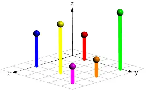
How about this xycomb with Asymptote?

xycomb

// Run on http://asymptote.ualberta.ca/
import three;
unitsize(1cm);
currentprojection=orthographic((1,1,.5),center=true,zoom=.95);
surface b=scale3(.2)*unitsphere;
pair[] xycomb={(0,1), (3,0), (4,4), (3,2), (2,4), (0,4)};
real[] h={1.5,2,1,3,1,3.5};
pen[] p={red,blue,magenta,yellow,orange,green};
pen q=linewidth(2mm)+opacity(1);
triple[] Mxy,M;
for (int i=0; i<xycomb.length; ++i){
M.push((xycomb[i].x,xycomb[i].y,h[i]));
Mxy.push((xycomb[i].x,xycomb[i].y,0));
draw(Mxy[i]--M[i],p[i]+q);
draw(shift(M[i])*b,p[i]);  
}

// grid on XY-plane import grid3; limits((-1,-1,0),(5,5,0)); grid3(XYXgrid,step=1,.5gray+.5white); draw(Label("$x$",EndPoint),-X--5X,Arrow3); draw(Label("$y$",EndPoint),-Y--5Y,Arrow3); draw(Label("$z$",EndPoint),O--3Z,Arrow3());

Appendix The option xcomb, ycomb, xbar, ybar are initially in TikZ (see Section 22.8 Smooth Plots, Sharp Plots, Jump Plots, Comb Plots and Bar Plots in the pgfmanual) that pgfplots is based on, I guess.

enter image description here

\documentclass[tikz,border=5mm]{standalone}
\begin{document}
\begin{tikzpicture}[thick]
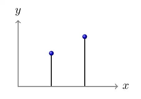
\draw plot[ycomb,mark=ball] coordinates{(1,1) (2,1.5)};
\draw[gray,<->] 
(3,0) node[right,black]{$x$}--(0,0)--(0,2) node[above,black]{$y$};
\end{tikzpicture}
\end{document}

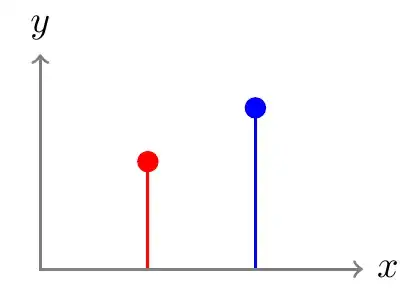
However, if one likes drawing directly with plain TikZ, then xcomb, ycomb, xbar, ybar can be ignored

enter image description here

\documentclass[tikz,border=5mm]{standalone}
\begin{document}
\begin{tikzpicture}[c/.style={circle,inner sep=2pt},thick]
\draw[red] (1,0)--+(90:1) node[c,fill=red]{};   
\draw[blue] (2,0)--+(90:1.5) node[c,fill=blue]{};
\draw[gray,<->] 
(3,0) node[right,black]{$x$}--(0,0)--(0,2) node[above,black]{$y$};      
\end{tikzpicture}
\end{document}
Black Mild
  • 17,569
  • Thanks for the suggestions. but I 'm trying to keep everything inside tikz-pgf. I probably should have been clear about that. I suppose my question boils down to: "is there a way to get addplot3 to plot these from a function or a table? I can draw one from scratch if all I want is an example, BUT I want to be able to plot different functions. – TonyK Sep 18 '22 at 21:31
0

Based on feedback from here to a different but related question Is it possible to request a new plot type in pgfplots, and if so, how? I was able to modify one of the examples offered by @hpekristiansen to produce almost what I want, so this is almost an answer but it might be helpful to others -- besides, this is not appropriate for a comment. Question: How do I get rid of the end points at the top and bottom? I just want the line. I can live with this but maybe I can do better. Here is the code and the output is below:

\documentclass]{amsbook}
\usepackage{tikz}
\usepackage{pgfplots}
\pgfplotsset{compat=1.18}

\begin{document} \begin{tikzpicture} \begin{axis}[ view={110}{20}, width=10cm, height=10cm, grid=major, xmin=0,xmax=4, ymin=0,ymax=4, zmin=0,zmax=3, xtick={0,1,2,3,4}, ytick={0,1,2,3,4}, ylabel={$y$}, xlabel={$x$}, zlabel={$z$}, ] \addplot3 coordinates {(3,3,0) (3,3,1.5)}; \end{axis} \end{tikzpicture} \end{document}

enter image description here

TonyK
  • 625
  • 2
  • 9
  • Mmm, I was so excited to get this far that I didn't notice until now that the x-axis is backwards. Did I do that? – TonyK Sep 22 '22 at 18:55