6

I'm trying to graph the following function: y=\sqrt[5]{4x^4-x^5} didn't work out the first time, so I searched here for something that might help me and found this. Unfortunately, when I edited the code, it didn't work out for me, so I would ask if there is a way to generally graph a root function?

\documentclass[svgnames, border=3pt]{standalone}
\usepackage{pst-plot}
\usepackage{auto-pst-pdf}

\begin{document}

\psset{unit=2cm, algebraic, arrowinset=0.12, arrowsize=3pt, linejoin=1, showorigin=false}

\begin{pspicture}(-2.6,-2.6)(2.6,2.6) \psaxeslinecolor=LightSteelBlue, tickcolor=LightSteelBlue, arrows =->, ticksize=2pt -2pt, labelFontSize=\scriptstyle(-2.6,-2.6)(2.6,2.6)[$x$,-135] [$y$,-135] \uputdl{$O$} \psset{linewidth=1.2pt, linecolor=IndianRed, plotpoints=200, plotstyle=curve} \psplot{-2.6}{1}{-(x^5-4x^4)^(1/5)}% \psplot{1}{2.6}{(4x^4-x^5)^(1/5)}% \pslinelinewidth=0.6pt, linecolor=Crimson!50(2.8,2.467) \end{pspicture}

\end{document}

Output: by Geogebra

enter image description here

Zaragosa
  • 599
  • 6
    The question asks for a tikz code, but your example is a pspicture. Which of those do you want to be used by the answer? –  Jul 04 '23 at 01:39

3 Answers3

8

This is an attempt to answer the question, based on the assumptions that

  1. you want a tikz (rather than pstricks or pgfplots) code, and
  2. you wish to keep the elements of the pspicture.

A possible code accomplishing this is

\documentclass[tikz,svgnames, border=3pt]{standalone}
\begin{document}
\begin{tikzpicture}[>=stealth,line cap=round]
    \draw[->,LightSteelBlue] (-2.6,0) -- (2.6,0) node[below left]{$x$};
    \draw[->,LightSteelBlue] (0,-2.6) -- (0,2.6) node[below left]{$y$};
    \draw[line width=1.2pt,smooth,samples at={-2.6,-2.5,...,-0.1,-0.05,-0.01,0,0.01,0.05,0.1,0.2,...,2.6}] plot (\x,{\fpeval{(4*(\x)^4-(\x)^5)^(1/5)}});
    \draw[line width=0.6pt,Crimson!50](-2.8,-3.133)--(2.8,2.467);
\end{tikzpicture}
\end{document}

enter image description here

Note that

  • \fpeval is used since the basic pgf math is not too accurate when computing the root of a very small number,
  • in older TeX installations you will need to load xfp, and
  • samples at is employed to increase the density of samples around the origin.
  • when you employ samples at you not need to define domain (which is in your answer also wrong). smooth option is not needed (necessary) since you have sufficient number of sample that curve is smooth. – Zarko Jul 04 '23 at 06:05
  • 2
    @Zarko First point: agree and fixed it, thanks! Second point: I disagree. There is a difference between having straight segments and Bezier curves. smooth can give bad results when used incorrectly, but this is precisely the reason why I use samples at. –  Jul 04 '23 at 06:10
  • In your case `smooth˙ (by use of the spline function) only overwhelmed compilation. Result of compilation is not visible better. But this is up to you. – Zarko Jul 04 '23 at 06:38
  • 3
    @Zarko Many of those who has used piecewise linear plots on a projector are glad that there is a smooth option. This is particularly true if one uses blowups such as \framezoom or spy. It also does not affect the computation time notably on a modern computer, let alone overwhelms it. –  Jul 04 '23 at 06:44
  • I will not argue with you. BTW, , I'm well aware what smooth functions do. It is not general cure, it may cause wrong result in drawed functions too... – Zarko Jul 04 '23 at 06:51
  • Interesting, thank you very much for your answer, would it be possible for you to show me the different ways of plotting this with both tikz, pstricks or pgfplots? I am a beginner in this and I would like to see the different ways to make this graph and choose the one that seems most natural and understandable to me. Thanks in advance.

    I will attach an image made in Geogebra as a reference of the result and the domain that interests me.

    – Zaragosa Jul 06 '23 at 12:18
7

run with lualatex:

\documentclass[svgnames, border=3pt]{standalone}
\usepackage{pst-plot}
\begin{document}

\psset{unit=2cm, algebraic, arrowinset=0.12, arrowsize=3pt, linejoin=1, showorigin=false}
\begin{pspicture}(-2.6,-2.6)(4.75,2.6) \psaxeslinecolor=LightSteelBlue, tickcolor=LightSteelBlue, arrows =->, ticksize=2pt -2pt, labelFontSize=\scriptstyle(-2.6,-2.6)(4.5,2.6)[$x$,-135] [$y$,-135] \uputdl{$O$} \psset{linewidth=2pt, linecolor=IndianRed, plotpoints=1200, plotstyle=line} \psplot{-2}{4}{(4x^4-x^5)^(0.2)}% \psplot[linecolor=blue]{4}{4.5}{-(abs(4x^4-x^5))^(0.2)}% \pslinelinewidth=0.6pt, linecolor=Crimson!50(2.8,2.467) \end{pspicture} \end{document}

enter image description here

enter image description here

user187802
  • 16,850
2

You've come to a point where you are seeing some of the limitations of mathematics in LaTeX. To be fair, LaTeX is for typesetting and you shouldn't expect it to take the place of Geogebra. This is an opportunity to assess how much complicated mathematics you will be using in LaTeX otherwise the problem of graphing the 5th root today can become pgfplots: problem with convergence of addplot on (sin(x) - x cos(x)) / x^3. As I say in my answer there, "The sledgehammer that will solve most any problem is a computer algebra system (CAS). The sagetex package gives you access to an open source CAS called Sage as well as Python programming.". A CAS has a steeper learning curve but can solve more problems: integration, derivatives, differential equations, matrix inverses, graph theory, etc. and Python gives you a powerful programming language to replace some of the more dated LaTeX programming that many here have mastered.

Here is a sagetex solution to your problem:

\documentclass{article}
\usepackage{sagetex,xcolor,pgfplots}
\pgfplotsset{compat=1.16}
\begin{document}
\begin{sagesilent}
LowerX = -5
UpperX = 5
LowerY = -5
UpperY = 5
step = .01
t = var('t')
g(t)= real_nth_root(4*t^4-t^5, 5)

x_coords = [t for t in srange(LowerX,UpperX,step)] y_coords = [g(t).n(digits=6) for t in srange(LowerX,UpperX,step)]

output = r"" output += r"\begin{tikzpicture}[scale=1.0]" output += r"\begin{axis}[xmin=%f,xmax=%f,ymin= %f,ymax=%f,width=10cm,"%(LowerX,UpperX,LowerY, UpperY) output += r"xlabel=$x$,ylabel=$y$,axis x line=middle,axis y line=middle]" output += r"\addplot[thin, blue, unbounded coords=jump] coordinates {" for i in range(0,len(x_coords)-1): if (y_coords[i])<LowerY or (y_coords[i])>UpperY: output += r"(%f , inf) "%(x_coords[i]) else: output += r"(%f , %f) "%(x_coords[i],y_coords[i]) output += r"};" output += r"\end{axis}" output += r"\end{tikzpicture}" \end{sagesilent} \sagestr{output} \end{document}

The output in Cocalc is:

enter image description here

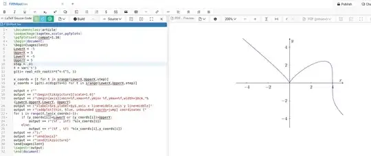
A brief explanation: sagesilent environment is work behind the scenes that doesn't get printed until you tell it. LowerX = -5, UpperX = 5, LowerY = -5, UpperY=5 sets up the parameters of what will be on the screen, step = .01 sets up the spacing between x-values. g(t)= real_nth_root(4*t^4-t^5, 5) indicates the 5th root of your function will be graphed but since there are 5 such roots over the complex number field, we specify that the real valued answer will be used. x_coords = [t for t in srange(LowerX,UpperX,step)] creates a list of the specific x-coordinates that will be used: -5, -4.99, -4.98, ..., 4.99 (Python doesn't include the last number. You can modify to UpperX+step to go to 5.00). The y-coordinates get calculated using 6 significant digits. The picture is created as a text string because sagetex runs as a 3-step compilation process. If you search this site for sagetex you can find more explanation on this. \sagestr{output} takes the work created in sagesilent so that on the third step of compilation all the calculations/details from Python/Sage get typeset. The for-loop for i in range(0,len(x_coords)-1): checks that the y-value is on the screen. If it isn't the y-value is infinity and won't be plotted. Otherwise it will be plotted.

LaTeX, a CAS, and Python programming can help you solve and typeset most anything. However, the CAS Sage is not part of your distribution. The easiest way to access it is through a free Cocalc account. It's also possible to download Sage to your computer and get it to work with your LaTeX distribution. That takes more time and can be more problematic. It requires more maintenance as well: as Sage and LaTeX update on different schedules, that coordination can break. Working on Cocalc means they make sure everything stays up to date and works. If you don't need the mathematical power of a CAS then other solutions, such as lua, are probably more appropriate.

DJP
  • 12,451