11

I am trying to plot the function f(x) = (sin(x) - x cos(x)) / x^3 using the pgfplots code

    \begin{tikzpicture}
        \begin{axis}[]
            \addplot[domain = 0:14,smooth,samples=500, thick] {(sin(deg(x))- x * cos(deg(x))) / (x^3)};
        \end{axis}
    \end{tikzpicture}

The code works, however has problems converging at x = 0 resulting in an incorrect graph close to the origin: enter image description here

Is there anything I can do to circumvent this issue, e.g. by increasing the precision of the addplot command?

Thanks in advance!

Black Mild
  • 17,569

6 Answers6

16

If you want to go all the way to 0, then I would suggest using the first terms of the Taylor expansion near 0

Sample output

\documentclass{article}

\usepackage{pgfplots}

\begin{document} \begin{tikzpicture} \begin{axis}[] \addplot[domain = 2:15,smooth,samples=500, thick] {(sin(deg(x))- x * cos(deg(x)) ) / (x^3) }; \addplot[domain = 0:2,smooth,samples=500, thick, red] {(1/3 - x^24/5! + x^46/7! - x^6*8/9!}; \end{axis} \end{tikzpicture} \end{document}

Here I have coloured the plot of the Taylor expansion red. Also I have exaggerated the range where the Taylor expansion is used, placing the swap over at 2. Something smaller than 1, e.g. 0.5, would be more sensible.

Andrew Swann
  • 95,762
12

The problem is that the numerator is cubic near 0 and this goes beyond the arithmetic capabilities of PGF.

You can use pgfmath-xfp that deals better with floating point calculations. Note that you need to avoid computing at 0, but it's not a real problem.

\documentclass{article}
\usepackage{pgfplots}
\usepackage{pgfmath-xfp}
\pgfplotsset{compat=1.18}

\begin{document}

\begin{tikzpicture} \pgfmxfpdeclarefunction{foo}{1}{(sin(#1)-(#1)*cos(#1))/(#1)^3} \begin{axis}[] \addplot[domain = 0.001:14,smooth,samples=500, thick] {foo(x)}; \end{axis} \end{tikzpicture}

\end{document}

enter image description here

You might also define the function at 0, but it's not worth the pain:

\pgfmxfpdeclarefunction{foo}{1}{ #1=0 ? 1/3 : (sin(#1)-(#1)*cos(#1))/(#1+(#1=0?1:0))^3}

The correction in the denominator is necessary because both expressions are computed, so I make the denominator to be 1 when x=0.

egreg
  • 1,121,712
12

You can use the gnuplot option which gives much more precision. The compilation must include the -shell-escape option. The gnuplot command must be available from your box.

\documentclass{article}
\usepackage{tikz,pgfplots}

\begin{document} \begin{tikzpicture} \begin{axis}[] \addplot[domain = 0:14,smooth,samples=500, thick] gnuplot {(sin(x)- x * cos(x)) / (x^3)}; % ^^^^^^^ \end{axis} \end{tikzpicture} \end{document}

graphe

Other solution:

You can create a table with any software or programmating language able to do that and save the data in a data file (for instance http://ix.io/3PQw) and use the table keyword

\documentclass{article}
\usepackage{tikz,pgfplots}

\begin{document} \begin{tikzpicture} \begin{axis}[] \addplot[smooth, thick] table {data.dat}; % ^^^^^^^ \end{axis} \end{tikzpicture} \end{document}

This solution does not need -shell-escape but involves slightly slower compilation than the first. However the first solution is three to four times faster than the solution with pgfmath-xfp and nearly five times faster than Andrew Swann's solution. This may matter on some large documents with lots of calculations.

gigiair
  • 1,812
6

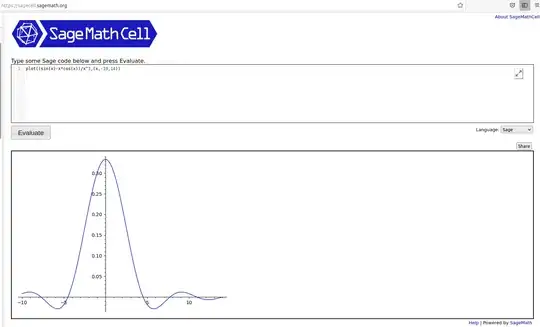
There comes a time in LaTeX plotting where you have to decide the pros and cons of your method. While LaTeX can handle the basics well, as @egreg points out, the cubic is well beyond the capability of PGF. He goes on to point out pgfmath-xfp can deal with floating point issues even better. @Andrew Swann shows that taking advantage of the Taylor series expansion can get you the results you want as well. The more plotting you have to do the more likely you will come up against limitations. The sledgehammer that will solve most any problem is a computer algebra system (CAS). The sagetex package gives you access to an open source CAS called Sage as well as Python programming. Sage is like Mathematica, except it's free.You can access it for free through a Sage Cell Server. Type the following plot((sin(x)-x*cos(x))/x^3,(x,-10,14)), press Evaluate and get the result below: enter image description here

A CAS has the power to handle the mathematics more accurately. You can use the CAS to generate the points, and use tizk to plot them via the sagetex package.

Here is some sample code:

\documentclass[11pt,border=1mm]{standalone}
\usepackage{sagetex}
\usepackage[usenames,dvipsnames]{xcolor}
\usepackage{pgfplots}
\pgfplotsset{compat=1.16}
\begin{document}
\begin{sagesilent}
LowerX = 0.001
UpperX = 14
LowerY = -.1
UpperY = .35
step = .1
t = var('t')
g(x)= (sin(x)-x*cos(x))/x^3

x_coords = [t for t in srange(LowerX,UpperX,step)] y_coords = [g(t).n(digits=6) for t in srange(LowerX,UpperX,step)]

output = r"" output += r"\begin{tikzpicture}[scale=1.0]" output += r"\begin{axis}[xmin=%f,xmax=%f,ymin= %f,ymax=%f,width=10cm]"%(LowerX,UpperX,LowerY, UpperY) output += r"\addplot[thin, blue, unbounded coords=jump] coordinates {" for i in range(0,len(x_coords)-1): if (y_coords[i])<LowerY or (y_coords[i])>UpperY: output += r"(%f , inf) "%(x_coords[i]) else: output += r"(%f , %f) "%(x_coords[i],y_coords[i]) output += r"};" output += r"\end{axis}" output += r"\end{tikzpicture}" \end{sagesilent} \sagestr{output} \end{document}

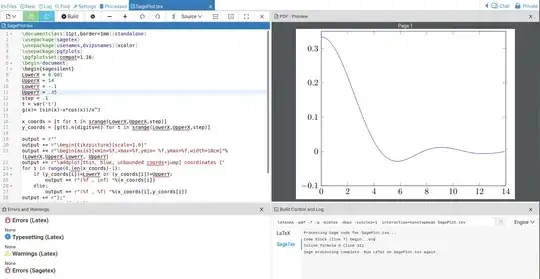
The output, running in Cocalc is below: enter image description here

The drawback is Sage is not part of a LaTeX distribution. The easiest way to work with it is through a free Cocalc account. Less easy is to install Sage on your computer and get it to work with your LaTeX distribution. I've had some problems doing this in Windows but Linux hasn't been difficult.

If you're using mathematics frequently, Sage and sagetex are worth the time and effort learning. Search this site for sagetex examples. The Cantor function, here and the Weierstrass function here can be plotted without much difficulty.

The documentation for sagetex is here.

DJP
  • 12,451
5

Just to complete Andrew's answer, you can use x ? y : z notation to make it with only one \addplot:

\documentclass{standalone}

\usepackage{pgfplots}

\begin{document} \begin{tikzpicture} \begin{axis}[] \addplot[domain = 0:15,smooth,samples=500, thick] { abs(x)>0.5 ? (sin(deg(x))- x * cos(deg(x)) ) / (x^3) : (1/3 - x^24/5! + x^46/7! - x^6*8/9! }; \end{axis} \end{tikzpicture} \end{document}

From pgfmanual: x ? y : z ? and : are special operators which can be used as a shorthand for if x then y else z inside the parser

4

Just notice that Asymptote, with high accuracy, is a straight way to draw such functions. I add f(0)=1/3 (see this Wolfram Alpha link), then draw its graph as usual, no tricks. operator.. is used for this smooth function.

enter image description here

// http://asymptote.ualberta.ca/
unitsize(5mm,20cm);
import graph;
real f(real x){
if (x==0) return 1/3;
else  return (sin(x) - x * cos(x)) / (x^3);
}

path p=graph(f,0,15,operator..); //path p=graph(f,-15,15,operator..); draw(p,red+1pt);

xaxis("$x$",BottomTop,LeftTicks); yaxis("$y$",LeftRight,RightTicks(trailingzero));

shipout(bbox(5mm,invisible));

enter image description here

Black Mild
  • 17,569