Intuition behind the Monte carlo method

Question

Addendum Thanks to Schrodinger's cat answer, I'm now able to produce the graph below. It shows that if you don't want to underestimate low probability events for further simulations, you really need to simulate loads of uniform numbers...

Original question I'd like to show graphically the intuition of the Monte Carlo method. The idea is the more random numbers you use, the more the simulated distributions below are populated. Once you reach a number large enough (500? 1000? more ?), these simulated distributions don't present any "hole" and can be used to simulate other processes.

The marks are each initial random number projected first horizontally on the cumulative and then projected vertically on the density. I used 40 random numbers in this example and highlighted 4 colored points just to show the projection sequence.

So far

I have the random numbers between [0,1]
I('d like to) project them on the y axis of the Cumulative normal distribution
which corresponds to a point on the normal density.

MWE does not connect the dots and does not make correspond the random numbers and their projections on the graphs. Probably because I need the inverse normal cumulative but based on Equation 8 at https://core.ac.uk/download/pdf/41787448.pdf gives a simple expression for the best logistic fit for the cumulative normal distribution: $\phi(z) \approx \frac{1}{(1 + e^{-1.702z})}$ %% (i use a more accurate one in MWE but it'd be sufficient for the example. The inverse : $z(\phi) \approx - \frac{ln (\frac{1}{\phi}-1)}{1.702}$

Here is MWE so far, Based on pedagogic-graph-of-lognormal-distribution

\documentclass{standalone}
\usepackage{tikz}

\usepackage{pgfplots}
\usepgfplotslibrary{groupplots,fillbetween}

\def\m{0}
\def\SIG{1}
\def\NumRand{50}

\begin{document}
\begin{tikzpicture}[declare function={
g(\x)= 1/(sqrt(2*pi))*exp(-0.5*(pow((\x-\m),2))/(2*\SIG^2));
h(\x)=1/(1 + exp(-0.07056*((\x-\m)/\SIG)^3 - 1.5976*(\x-\m)/\SIG));
}]

\begin{groupplot}[group style={
            group size=2 by 2, horizontal sep=0pt, vertical sep=0pt,
            xticklabels at=edge bottom},  legend pos=south east,
%       grid=both
        ]
        \nextgroupplot[group/empty plot]

        %---- top right    -------------------
        \nextgroupplot[]    
        \addplot[name path=BL1,only marks,very thick,color=red,domain=-4:4,samples=\NumRand] ({x},{g(x)});
        \addlegendentry{$\mathcal{N}(0,1)$}

        %----  bottom left  -------------------
        \nextgroupplot  
        \addplot+[only marks,fill=blue!60, opacity= 0.5, samples=\NumRand,domain=-0.1:0.1] (0,rnd);
        \addlegendentry{Uniform random numbers}             
        %----  bottom right    -------------------
        \nextgroupplot[]
        \addplot[name path=BR1,only marks, color=red!50, domain=-4:4, samples=\NumRand] ({x},{h(x)});
        \addlegendentry{Normal cumulative}
        \end{groupplot}

\end{tikzpicture}
\end{document}

The accuracy of the cumulative normal expression is discussed at length in the referenced article. There are more accurate expressions there, but they're not quite so easy to invert and require more computational overhead. This one can be used for coding purposes where you want to generate "random" samples from a normal distribution

On a tangent note, the best intuition for Monte Carlo I have looks somewhat differently. Draw a complex shape inside a simple square. Bombard the square with random points. Count points inside the complex shape and in total. Their relation times the area of the square is an approximation of the area of the complex shape. — Oleg Lobachev, Apr 18 '20 at 22:05
I agree with you @OlegLobachev. As in https://tex.stackexchange.com/questions/244488/monte-carlo-method-drawing. With the current approach I tried to show my students that, as long as (1) you give me enough random numbers between 0 and (2) an (inversible) cumulative distribution, I can implicitly recreate a density that can be used for other simulations purposes. Next step is to adapt the code with an Exponential or a log-normal distribution. — JeT, Apr 18 '20 at 22:15

score 5 · Accepted Answer · 2020-04-18T17:51:49.817

EDIT: You may be asking for this:

\documentclass[tikz,border=3mm]{standalone}
\usepackage{pgfplots}
\pgfplotsset{compat=1.17}
\usepgfplotslibrary{groupplots}
\begin{document}
\begin{tikzpicture}[declare function={
g(\x,\m,\SIG)= 1/(sqrt(2*pi))*exp(-0.5*(pow((\x-\m),2))/(2*\SIG^2));
h(\x,\m,\SIG)=1/(1 + exp(-0.07056*((\x-\m)/\SIG)^3 - 1.5976*(\x-\m)/\SIG));
phi(\z)=1/(1+exp(-1.702*\z));
z(\phi)=-ln((1-\phi)/\phi)/1.702;
}]
\edef\m{0}
\edef\SIG{1}
\edef\NumRand{50}
\newcommand\RandDist[1]{\edef\irun{0}%
\pgfmathsetmacro{\mysum}{0}%
\edef\lstcoords{}%
\edef\lstcm{}%
\edef\lstgf{}%
\loop
\pgfmathsetmacro{\myrnd}{rnd}%
\pgfmathsetmacro{\mysum}{\mysum+\myrnd}%
\edef\lstcoords{\lstcoords (#1,\myrnd)}%
\pgfmathsetmacro{\myz}{z(\myrnd)}%
\edef\lstcm{\lstcm (\myz,\myrnd)}%
\pgfmathsetmacro{\myg}{g(\myz,\m,\SIG)}%
\edef\lstgf{\lstgf (\myz,\myg)}%
\edef\irun{\the\numexpr\irun+1}%
\ifnum\irun<\NumRand\relax
\repeat
}
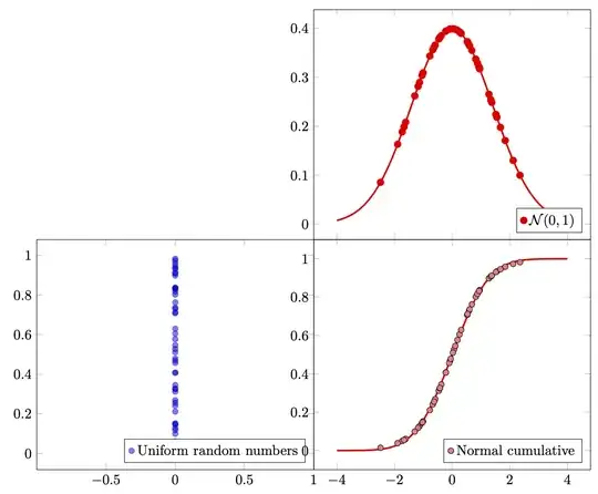
\RandDist{0}
\begin{groupplot}[group style={
            group size=2 by 2, horizontal sep=0pt, vertical sep=0pt,
            xticklabels at=edge bottom},  legend pos=south east,
%       grid=both
        ]
        \nextgroupplot[group/empty plot]

        %---- top right    -------------------
        \nextgroupplot[]    
        \addplot[forget plot,very thick,color=red,domain=-4:4,samples=\NumRand+1] ({x},{g(x,\m,\SIG)});
        \addplot[only marks,very thick,color=red] 
         coordinates {\lstgf};
        \addlegendentry{$\mathcal{N}(0,1)$}

        %----  bottom left  -------------------
        \nextgroupplot  
        \addplot+[only marks,fill=blue!60, opacity= 0.5]
            coordinates {\lstcoords};
        \addlegendentry{Uniform random numbers}             
        %----  bottom right    -------------------
        \nextgroupplot[]
        \addplot[forget plot,very thick,color=red, domain=-4:4, samples=\NumRand+1] ({x},{h(x,\m,\SIG)});
        %\addplot[orange, domain=-4:4,]({x},{phi(x)});
        \addplot[only marks,fill=red!50]  coordinates {\lstcm};
        \addlegendentry{Normal cumulative}
        \end{groupplot}

\end{tikzpicture}
\end{document}

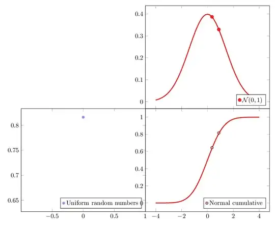
You can animate it.

\documentclass[tikz,border=3mm]{standalone}
\usepackage{pgfplots}
\pgfplotsset{compat=1.17}
\usepgfplotslibrary{groupplots}
\tikzset{declare function={
g(\x,\m,\SIG)= 1/(sqrt(2*pi))*exp(-0.5*(pow((\x-\m),2))/(2*\SIG^2));
h(\x,\m,\SIG)=1/(1 + exp(-0.07056*((\x-\m)/\SIG)^3 - 1.5976*(\x-\m)/\SIG));
phi(\z)=1/(1+exp(-1.702*\z));
z(\phi)=-ln((1-\phi)/\phi)/1.702;
}}
\begin{document}
\begingroup
\edef\m{0}
\edef\SIG{1}
\edef\NumRand{50}
\newcommand\RandDist[1]{\edef\irun{0}%
\pgfmathsetmacro{\mysum}{0}%
\edef\lstcoords{}%
\edef\lstcm{}%
\edef\lstgf{}%
\loop
\pgfmathsetmacro{\myrnd}{rnd}%
\pgfmathsetmacro{\mysum}{\mysum+\myrnd}%
\edef\lstcoords{\lstcoords (#1,\myrnd)}%
\pgfmathsetmacro{\myz}{z(\myrnd)}%
\edef\lstcm{\lstcm (\myz,\myrnd)}%
\pgfmathsetmacro{\myg}{g(\myz,\m,\SIG)}%
\edef\lstgf{\lstgf (\myz,\myg)}%
\edef\irun{\the\numexpr\irun+1}%
\ifnum\irun<\NumRand\relax
\repeat
}
\RandDist{0}
\pgfplotsinvokeforeach{1,...,\NumRand}{\begin{tikzpicture}
\begin{groupplot}[group style={
            group size=2 by 2, horizontal sep=0pt, vertical sep=0pt,
            xticklabels at=edge bottom},  legend pos=south east,
%       grid=both
        ]
        \nextgroupplot[group/empty plot]

        %---- top right    -------------------
        \nextgroupplot[]    
        \addplot[forget plot,very thick,color=red,domain=-4:4,samples=\NumRand+1] ({x},{g(x,\m,\SIG)});
        \addplot[only marks,very thick,color=red,
            x filter/.expression={(\coordindex >#1 ? nan : x)}] 
         coordinates {\lstgf};
        \addlegendentry{$\mathcal{N}(0,1)$}

        %----  bottom left  -------------------
        \nextgroupplot  
        \addplot+[only marks,fill=blue!60, opacity= 0.5,
            x filter/.expression={(\coordindex >#1 ? nan : x)}]
            coordinates {\lstcoords};
        \addlegendentry{Uniform random numbers}             
        %----  bottom right    -------------------
        \nextgroupplot[]
        \addplot[forget plot,very thick,color=red, domain=-4:4, samples=\NumRand+1] ({x},{h(x,\m,\SIG)});
        %\addplot[orange, domain=-4:4,]({x},{phi(x)});
        \addplot[only marks,fill=red!50,
            x filter/.expression={(\coordindex >#1 ? nan : x)}]  coordinates {\lstcm};
        \addlegendentry{Normal cumulative}
        \end{groupplot}
\end{tikzpicture}}
\endgroup
\end{document}

However, I am not sure about the interpretation.

ORIGINAL ANSWER: This may be missing the whole point of this exercise. All this does is to generate a set of random distributions of points, computes their averages and plots the distribution of averages. And it varies the number of sets in an animation.

\documentclass[tikz,border=3mm]{standalone}
\usepackage{pgfplots}
\pgfplotsset{compat=1.17}
\usepgfplotslibrary{groupplots,fillbetween}
\begin{document}
\foreach \X in {4,8,...,80}
{\begin{tikzpicture}
\edef\NumRand{50}
\edef\NumSamples{\X}
\edef\NumBins{25}
\edef\irun{0}%
\loop
\expandafter\edef\csname NumBin\irun\endcsname{0}%
\edef\irun{\the\numexpr\irun+1}%
\ifnum\irun<\NumBins\relax
\repeat
\newcommand\RandDist[1]{\edef\irun{0}%
\pgfmathsetmacro{\mysum}{0}%
\edef\lstcoords{}%
\loop
\pgfmathsetmacro{\myrnd}{rnd}%
\pgfmathsetmacro{\mysum}{\mysum+\myrnd}%
\edef\lstcoords{\lstcoords (##1,\myrnd)}%
\edef\irun{\the\numexpr\irun+1}%
\ifnum\irun<\NumRand\relax
\repeat
}
\pgfplotsforeachungrouped\isample in{0,...,\the\numexpr\NumSamples-1}
{\pgfmathsetmacro{\xsample}{2*\isample/\NumSamples-1}%
\RandDist{\xsample}%
\expandafter\edef\csname lstpst\isample\endcsname{\lstcoords}%
\pgfmathsetmacro{\avg}{\mysum/\NumRand}%
\expandafter\edef\csname avg\isample\endcsname{(\xsample,\avg)}%
\pgfmathtruncatemacro{\nBin}{25*\avg}%
\edef\currbin{\csname NumBin\nBin\endcsname}%
\expandafter\edef\csname NumBin\nBin\endcsname{\the\numexpr\currbin+1}%
}
\edef\lstbars{}%
\edef\irun{0}%
\loop
\edef\lstbars{\lstbars (\irun,\csname NumBin\irun\endcsname)}%
\edef\irun{\the\numexpr\irun+1}%
\ifnum\irun<\NumBins\relax
\repeat
%\typeout{\lstcoords,\mysum,\lstbars}
\begin{groupplot}[group style={
            group size=2 by 2, horizontal sep=2em, vertical sep=0pt,
            xticklabels at=edge bottom},  legend pos=south east,
%       grid=both
        ]
        \nextgroupplot[title=samples]
        \edef\temp{\noexpand\addplot[only marks,mark=*,fill=blue!60, opacity= 0.5]
        coordinates {\csname lstpst0\endcsname};
        \noexpand\addlegendentry{samples}
        \noexpand\addplot[only marks,mark=square*,fill=red!60]
        coordinates {\csname avg0\endcsname};
        \noexpand\addlegendentry{average}}
        \temp       
        \pgfplotsinvokeforeach{1,...,\the\numexpr\NumSamples-1}
        {\edef\temp{\noexpand\addplot[forget plot,only marks,mark=*,fill=blue!60, opacity= 0.5]
        coordinates {\csname lstpst##1\endcsname};
        \noexpand\addplot[forget plot,only marks,mark=square*,fill=red!60]
        coordinates {\csname avg##1\endcsname};}
        \temp}
%        \addlegendentry{Uniform random numbers}             
        %---- top right    -------------------
        \nextgroupplot[title=distribution of averages,
            xtick={0,...,\NumBins},xticklabel=\empty] 
        \addplot[ybar,bar width=pi*1pt,fill=blue] coordinates{\lstbars};   
        %----  bottom left  -------------------
        \end{groupplot}

\end{tikzpicture}}
\end{document}

Intuition behind the Monte carlo method

1 Answers1