3

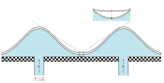
Is it possible to draw like an inset style figure but just using tikz ? Obviously, I am trying to use the zoom effect by focusing on a particular region of a scheme but I want to achieve is :

  • Inside the inset figure, I want to show a portion of the global profile in the red dot and then add the shape of the same profile but in the point at the end of the arrow. So these two profiles need to be present only in the zoomed region not in the whole picture : this is mainly why I am struggling here

How do you think it would be possible to achieve that ?

Thank you for your comments,

Best regards.

Code :

\documentclass{article}
\usepackage[utf8]{inputenc}

%%%%%%%%MATHS%%%%%%%%%%%%% \usepackage{amsmath} \usepackage{amsfonts} \usepackage{color} %red, green, blue, yellow, cyan, magenta, black, white

%%%%%%%%GEOMETRIE%%%%%%%%%%% \usepackage{geometry} \usepackage{layout}

%%%AXIS%%%% \usepackage{pgfplots} \pgfplotsset{compat=newest}

%%%%%%%%SECTIONS/AGENCEMENT%%% \usepackage{pgf, tikz, adjustbox} \usepgfplotslibrary{fillbetween} \usetikzlibrary{calc} \usetikzlibrary{spy} \usetikzlibrary{patterns, matrix, positioning} \usetikzlibrary{arrows.meta, patterns.meta }

\usepackage[framemethod=tikz]{mdframed} % breakable frames and coloured boxes \usetikzlibrary{decorations.pathmorphing} %%%%%%%%GAUSSIAN%%%%%%%%%%%% \pgfmathdeclarefunction{gauss}{1}{% \pgfmathparse{3*exp(-(#1/2.5)^2)} }

\begin{document}

\begin{figure}[h] \centering \begin{tikzpicture}[spy using outlines, dot/.style = {circle, fill, inner sep=2.0pt, node contents={}}, scale = 1, s/.style={shift=(0:9)}] \fill [cyan!20] plot[domain= -4:13, samples=100] (\x, {gauss(\x)+gauss(\x-9}) |- (-4,0) -| cycle; \filldraw[fill=pink!20, thick] plot[domain=-4:13, samples=100] (\x, {gauss(\x)+gauss(\x-9)}) -- plot[domain=13:-4, samples=100] (\x, {gauss(\x)+gauss(\x-9)+0.2}) -- cycle; \path[fill=cyan!20] (-0.5,-2) -- (-0.5,0) -- (0.5,0) -- (0.5,-2) -- (-0.5,-2); \path[fill=cyan!20] (8.5,-2) -- (8.5,0) -- (9.5,0) -- (9.5,-2) -- (8.5,-2); \draw[black,thick] (0.5,-2) -- (0.5,0) -- (8.5,0) -- (8.5,-2);
\draw[black,thick] (-0.5,-2) -- (-0.5,0) -- (-4,0);
\draw[black,thick] (9.5,-2) -- (9.5,0) -- (13,0);
\draw[dashed,red, stealth-stealth, thick] (-0.5,-2.25) -- node[below,scale=0.75] {$e \sim 1 \ mm$} (0.5,-2.25); \draw yshift=-0.25cm, -latex -- node [fill=cyan!20,scale=0.75] {$Q_1$} (0,0); \draw yshift=-0.25cm, -latex -- node [fill=cyan!20,scale=0.75] {$Q_2$} (9,0); \spy [blue,draw,height=3cm,width=7cm,magnification=2,connect spies] on (4.5,0.85) in node at (4.5,5); % ZOOM EFFECT \coordinate [red] (A) at (4.5,0.45) ; \coordinate [red] (B) at (4.5,1.35) ; \draw[dashed,-stealth,black!30!red,thick] (A) to (B) ; \path (4.5,0.45) node[black!30!red,dot] ; \end{tikzpicture} \end{figure} \end{document}

Image : enter image description here

EDIT

I am trying to improve my previous attempt and I considered using a mixed solution as suggested in these posts : post1 and post2 by implementing a savebox feature and link 2 different graphs together

I am still not satisfied with it : for some reason I don't manage to understand the size of the node that I create for the second picture above that I want to be centered in the middle of the first main graph but didn't succeed to do that...

Second code :

\documentclass{article}
\usepackage[utf8]{inputenc}

%%%%%%%%MATHS%%%%%%%%%%%%% \usepackage{amsmath} \usepackage{amsfonts}

%%%%%%%%GEOMETRIE%%%%%%%%%%% \usepackage{geometry} \usepackage{layout}

%%%AXIS%%%% \usepackage{pgfplots} \pgfplotsset{compat=newest}

%%%%%%%%SECTIONS/AGENCEMENT%%% \usepackage{pgf, tikz, adjustbox} \usepgfplotslibrary{fillbetween} \usetikzlibrary{calc} \usetikzlibrary{spy} \usetikzlibrary{patterns, matrix, positioning} \usetikzlibrary{arrows.meta, patterns.meta }

\usepackage[framemethod=tikz]{mdframed} % breakable frames and coloured boxes \usetikzlibrary{decorations.pathmorphing} %%%%%%%%GAUSSIAN%%%%%%%%%%%% \pgfmathdeclarefunction{gauss}{1}{% \pgfmathparse{3exp(-(#1/2.5)^2)} } \pgfmathdeclarefunction{gaussquatre}{1}{% \pgfmathparse{3exp(-(#1/1.5)^2)} }

%%%%% DOCUMENT%%%%%% \begin{document}

\newsavebox\Graphone \sbox\Graphone{\begin{tikzpicture}[spy using outlines, dot/.style = {circle, fill, inner sep=1.5pt, node contents={}}, scale = 1, s/.style={shift=(0:9)}] \fill [cyan!20] plot[domain= -4:13, samples=100] (\x, {gauss(\x)+gauss(\x-9}) |- (-4,0) -| cycle; \filldraw[fill=pink!20, thick] plot[domain=-4:13, samples=100] (\x, {gauss(\x)+gauss(\x-9)}) -- plot[domain=13:-4, samples=100] (\x, {gauss(\x)+gauss(\x-9)+0.2}) -- cycle; \path[fill=cyan!20] (-0.5,-2) -- (-0.5,0) -- (0.5,0) -- (0.5,-2) -- (-0.5,-2); \path[fill=cyan!20] (8.5,-2) -- (8.5,0) -- (9.5,0) -- (9.5,-2) -- (8.5,-2); \draw[black,thick] (0.5,-2) -- (0.5,0) -- (8.5,0) -- (8.5,-2);
\draw[black,thick] (-0.5,-2) -- (-0.5,0) -- (-4,0);
\draw[black,thick] (9.5,-2) -- (9.5,0) -- (13,0);
\draw[dashed,red, stealth-stealth, thick] (-0.5,-2.25) -- node[below,scale=0.75] {$e \sim 1 \ mm$} (0.5,-2.25); \draw yshift=-0.25cm, -latex -- node [fill=cyan!20,scale=0.75] {$Q_1$} (0,0); \draw yshift=-0.25cm, -latex -- node [fill=cyan!20,scale=0.75] {$Q_2$} (9,0); \draw[black, pattern = checkerboard] (-0.5,-.5) -- (-0.5,0) -- (-4,0) -- (-4,-.5) -- cycle; \draw[black, pattern = checkerboard] (9.5,-.5) -- (9.5,0) -- (13,0) -- (13,-.5) -- cycle; \draw[black, pattern = checkerboard] (0.5,-.5) -- (0.5,0) -- (8.5,0) -- (8.5,-.5) -- cycle;
\end{tikzpicture}}

\newsavebox\Graphbis \sbox\Graphbis{\begin{tikzpicture}[spy using outlines, dot/.style = {circle, fill, inner sep=1.5pt, node contents={}}, scale = 1, ] \fill [cyan!20] plot[domain= 2.5:6.5, samples=100] (\x, {gauss(\x)+gauss(\x-9}) |- (-4,0) -| cycle; \filldraw[fill=pink!20, thin] plot[domain=2.5:6.5, samples=100] (\x, {gauss(\x)+gauss(\x-9)}) -- plot[domain=6.5:2.5, samples=100] (\x, {gauss(\x)+gauss(\x-9)+0.1}) -- cycle; \filldraw[fill=pink!20, thin] plot[domain=2.5:6.5, samples=100] (\x, {gaussquatre(\x)+gaussquatre(\x-9)+1}) -- plot[domain=6.5:2.5, samples=100] (\x, {gaussquatre(\x)+gaussquatre(\x-9)+1.1}) -- cycle; \coordinate [red] (A) at (4.5,0.3) ; \coordinate [red] (B) at (4.5,1.1) ; \draw[dashed,-stealth,black!30!red,thin] (A) to (B) ; \path (4.5,0.285) node[black!30!red,dot] ; \end{tikzpicture}}

%%%%%%FIGURE \begin{figure}[h] \centering \begin{tikzpicture} \node(a){\usebox{\Graphone}}; \node(b)[inner sep=0pt,above = 0.5cm of a] {\phantom{\usebox{\Graphbis}}}; \node(c)[draw,minimum size=0.5cm, at=(a)]{}; \begin{scope}[thin,blue!40] \draw(c.north east) -- (b.south east); \draw(c.north west) -- (b.south west); \end{scope} \node [at=(b),inner sep=0pt,above = 0.5cm of a] {\usebox{\Graphbis}}; \end{tikzpicture} \end{figure}

\end{document}

Picture :
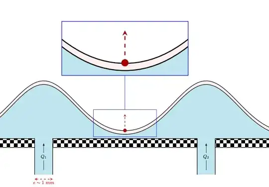
enter image description here

Waxler
  • 680
  • I suggest that you clean your preamble a bit. If you use pgfplots in your document, you don't need to load pgf and tikz as they are loaded anyways. Also, tikz loads the xcolor package which is the successor of the color package which you should therefore probably not load. – Jasper Habicht Mar 07 '24 at 16:36

1 Answers1

2

With Jasper Habicht's answer on the post2, we can use pic. I use a \clip and transform canvas. I use the math library to declare the scale. With the scale (\e), the coordinates are modified. The offset to find above the red point (4.5,0) is multiplied by (\e - 1)

\documentclass[border=3cm]{standalone}
%%%AXIS%%%%
\usepackage{pgfplots}
\pgfplotsset{compat=newest}
%%%%%%%%SECTIONS/AGENCEMENT%%%
\usetikzlibrary {math}%<-- added
\usetikzlibrary{patterns}
%%%%%%%%GAUSSIAN%%%%%%%%%%%%
\pgfmathdeclarefunction{gauss}{1}{%
    \pgfmathparse{3*exp(-(#1/2.5)^2)}
}
\pgfmathdeclarefunction{gaussquatre}{1}{%
    \pgfmathparse{3*exp(-(#1/1.5)^2)}
}

%%%%% DOCUMENT%%%%%% \begin{document} \tikzset{ dot/.style = {circle, fill, inner sep=2.0pt, node contents={}}, Graphone/.pic={ \fill [cyan!20] plot[domain= -4:13, samples=100] (\x, {gauss(\x)+gauss(\x-9}) |- (-4,0) -| cycle; \filldraw[fill=pink!20, thick] plot[domain=-4:13, samples=100] (\x, {gauss(\x)+gauss(\x-9)}) -- plot[domain=13:-4, samples=100] (\x, {gauss(\x)+gauss(\x-9)+0.2}) -- cycle; \path[fill=cyan!20] (-0.5,-2) -- (-0.5,0) -- (0.5,0) -- (0.5,-2) -- (-0.5,-2); \path[fill=cyan!20] (8.5,-2) -- (8.5,0) -- (9.5,0) -- (9.5,-2) -- (8.5,-2); \draw[black,thick] (0.5,-2) -- (0.5,0) -- (8.5,0) -- (8.5,-2);
\draw[black,thick] (-0.5,-2) -- (-0.5,0) -- (-4,0);
\draw[black,thick] (9.5,-2) -- (9.5,0) -- (13,0);
\draw[dashed,red, stealth-stealth, thick] (-0.5,-2.25) -- node[below,scale=0.75] {$e \sim 1 \ mm$} (0.5,-2.25); \draw yshift=-0.25cm, -latex -- node [fill=cyan!20,scale=0.75] {$Q_1$} (0,0); \draw yshift=-0.25cm, -latex -- node [fill=cyan!20,scale=0.75] {$Q_2$} (9,0); \coordinate [red] (A) at (4.5,0.45) ; \coordinate [red] (B) at (4.5,1.35) ; \draw[dashed,-stealth,black!30!red,thick] (A) to (B) ; \path (4.5,0.45) node[black!30!red,dot] ; }, Graphbis/.pic={ \fill [cyan!20] plot[domain= 2.5:6.5, samples=100] (\x, {gauss(\x)+gauss(\x-9}) |- (-4,0) -| cycle; \filldraw[fill=pink!20, thin] plot[domain=2.5:6.5, samples=100] (\x, {gauss(\x)+gauss(\x-9)}) -- plot[domain=6.5:2.5, samples=100] (\x, {gauss(\x)+gauss(\x-9)+0.1}) -- cycle; \filldraw[fill=pink!20, thin] plot[domain=2.5:6.5, samples=100] (\x, {gaussquatre(\x)+gaussquatre(\x-9)+1}) -- plot[domain=6.5:2.5, samples=100] (\x, {gaussquatre(\x)+gaussquatre(\x-9)+1.1}) -- cycle; \coordinate [red] (A) at (4.5,0.3) ; \coordinate [red] (B) at (4.5,1.1) ; \draw[dashed,-stealth,black!30!red,thin] (A) to (B) ; \path (4.5,0.285) node[black!30!red,dot] ; } } \tikzmath{ real \e; \e = 1.25; % scale } \begin{tikzpicture} \draw(0,0) grid (10,5);%<-- comment in the final document \pic (one) at (0,0) {Graphone}; \draw blue rectangle(7,2); \begin{scope}[transform canvas={xshift=-4.5cm*(\e-1),yshift=3cm,scale=\e}] \clip (2,0) rectangle(7,2); \pic (one) at (0,0) {Graphone}; \draw red--(10,2);% other code \end{scope} \end{tikzpicture}

\end{document}

enter image description here

EDIT: I will try to explain

With scale=2 the coordinates are also multiplied by 2

\begin{scope}[transform canvas={yshift=3cm,scale=2}]

enter image description here

With xshift=-4.5cm*(2-1) we shift to the left to be above the coordinate point (4.5,0.5)

enter image description here

For the connection between the graphone and the graphbis, I make a change of reference with shift={(4.5,0), I added variables (xone,yone) and (xbis,ybis) coordinated in the graphone.

Edit2: added shorten >=6pt and pos=0.5

\documentclass[border=5cm]{standalone}
%%%AXIS%%%%
\usepackage{pgfplots}
\pgfplotsset{compat=newest}
%%%%%%%%SECTIONS/AGENCEMENT%%%
\usetikzlibrary{patterns}
%%%%%%%%GAUSSIAN%%%%%%%%%%%%
\pgfmathdeclarefunction{gauss}{1}{%
    \pgfmathparse{3*exp(-(#1/2.5)^2)}
}
\pgfmathdeclarefunction{gaussquatre}{1}{%
    \pgfmathparse{3*exp(-(#1/1.5)^2)}
}
%%%%% DOCUMENT%%%%%%
\begin{document}
% \tikzset{
%   dot/.style = {circle, fill, inner sep=2.0pt, node contents={}},
% }
% \begin{tikzpicture}
%   \draw(0,0) grid (10,5);
%   \path (4.5,0.45) node[name=A,black!30!red,dot];
%   \path (2,0) node[name=B,black!30!red,dot];
%   \draw (A)--(B);
%   \begin{scope}[transform canvas={yshift=3cm,scale=2}]
%     \path (4.5,0.45) node[name=A,black!30!red,dot];
%     \path (2,0) node[name=B,black!30!red,dot];
%     \draw[red](A)--(B);    
%   \end{scope}
% \end{tikzpicture}

% \begin{tikzpicture} % \draw(0,0) grid (10,5); % \path (4.5,0.45) node[name=A,black!30!red,dot]; % \path (2,0) node[name=B,black!30!red,dot]; % \draw (A)--(B); % \begin{scope}[transform canvas={xshift=-4.5cm*(2-1),yshift=3cm,scale=2}] % \path (4.5,0.45) node[name=A,black!30!red,dot]; % \path (2,0) node[name=B,black!30!red,dot]; % \drawred--(B);
% \end{scope} % \end{tikzpicture}

\tikzset{ dot/.style = {circle, fill, inner sep=2.0pt, node contents={}}, Graphone/.pic={ \fill [cyan!20] plot[domain= -4:13, samples=100] (\x, {gauss(\x)+gauss(\x-9}) |- (-4,0) -| cycle; \filldraw[fill=pink!20, thick] plot[domain=-4:13, samples=100] (\x, {gauss(\x)+gauss(\x-9)}) -- plot[domain=13:-4, samples=100] (\x, {gauss(\x)+gauss(\x-9)+0.2}) -- cycle; \path[fill=cyan!20] (-0.5,-2) -- (-0.5,0) -- (0.5,0) -- (0.5,-2) -- (-0.5,-2); \path[fill=cyan!20] (8.5,-2) -- (8.5,0) -- (9.5,0) -- (9.5,-2) -- (8.5,-2); \draw[black,thick] (0.5,-2) -- (0.5,0) -- (8.5,0) -- (8.5,-2);
\draw[black,thick] (-0.5,-2) -- (-0.5,0) -- (-4,0);
\draw[black,thick] (9.5,-2) -- (9.5,0) -- (13,0);
\draw[dashed,red, stealth-stealth, thick] (-0.5,-2.25) -- node[below,pos=0.5,scale=0.75] {$e \sim 1 \ mm$} (0.5,-2.25); \draw yshift=-0.25cm,-latex,shorten >=6pt -- node [fill=cyan!20,scale=0.75] {$Q_1$} (0,0); \draw yshift=-0.25cm,-latex,shorten >=6pt -- node [fill=cyan!20,scale=0.75] {$Q_2$} (9,0); \coordinate [red] (A) at (4.5,0.45) ; \coordinate [red] (B) at (4.5,1.35) ; \draw[dashed,-stealth,black!30!red,thick] (A) to (B) ; \path (4.5,0.45) node[black!30!red,dot]; }, }

\begin{tikzpicture}[declare function={% s = 1.5;% scale ydecal=4cm;% offset of the clip }] \draw(0,0) grid (10,5);%<-- comment in the final document \pic (A) at (0,0) {Graphone}; \draw blue rectangle(7,2); %%%%%%%%% clip and tranlate \begin{scope}[transform canvas={xshift=-4.5cm*(s-1),yshift=ydecal,scale=s}] \clip (2,0)rectangle(7,2); \pic (B) at (0,0) {Graphone}; % add code \filldraw[fill=pink!20, thin] plot[domain=2.5:6.5, samples=100] (\x, {gaussquatre(\x)+gaussquatre(\x-9)+1})-- plot[domain=6.5:2.5, samples=100] (\x, {gaussquatre(\x)+gaussquatre(\x-9)+1.1}); \end{scope} %%%%% change the repere \begin{scope}[shift={(4.5,0)}, declare function={% xone=-2.5;% offset of the start of the arrow relative to the red point yone=2; xbis=-2.5; ybis=0; }] \draw->,very thick--(xbiss,ybiss+ydecal); \end{scope} \end{tikzpicture} \end{document}

enter image description here

pascal974
  • 4,652
  • Thank you for your complete answer. But I still have a problem figuring out the correct coordinates to use : for instance if I want to draw a line from the top left corner of the bottom blue rectangle to the bottom left of the upper rectangle how do you get the exact coordinates of the upper rectangle corners ? the line transform canvas={xshift=-4.5cm*(\e-1),yshift=3cm,scale=\e}lost me in terms of the translation done in cm... sorry for being redundant – Waxler Mar 08 '24 at 19:13
  • 1
    I tried to explain, I edited the answer – pascal974 Mar 09 '24 at 12:09
  • thank you again @pascal974 : I didn't know the scale is also applied to the coordinates also : this was tricky. Also, is there any reason that the arrows of the nodes Q_{1} and Q_{2} disappeared ? There is also a strange behavior of \epsilon \sim 1 mm which has moved to the right : and I can't force it back to its orignal position ! – Waxler Mar 10 '24 at 10:06
  • 1
    The arrows are hidden by the cyan color of the node. With shorten >=6pt, to add in \draw [yshift=-0.25cm,-latex,shorten >=6pt]. For the offset of \epsilon \sim 1 mm, by adding midway or pos=0.5 in node[below,pos=0.5,scale=0.75] (I don't know why). – pascal974 Mar 10 '24 at 10:59
  • well thanks again for your help ! indeed it seems like a strange offset happened even for the position of the Q_{1/2} nodes : I will use your suggestion to get rid of it. Thank you – Waxler Mar 10 '24 at 15:08